2.1.4 Distribution Function Models

To obtain simpler equation systems we can add further constraints on the distribution function. The following assumption can be justified in the framework of the diffusion approximation [GJK⁺04]: The symmetric part $f_S$ of $f$

$$f_S(x,k) = \frac{1}{2} (f(x,k) + f(x,-k))$$ (2.15)

is isotropic, that is

$$f_S(x,k) = f_S(x,\vert k\vert) .$$ (2.16)

We refer to it as the ``isotropy condition''.

Another model emerges from the first order approximation to a shifted Maxwellian [GJK⁺04]:

$$f(x,k) = g(x,\vert k\vert) + k_x h(x,\vert k\vert) .$$ (2.17)

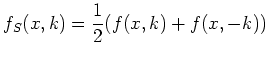
We call it the ``shifting'' assumption and refer to the class of functions as of ``linear-isotropic'' type. Distribution functions of this form also fulfill the isotropy condition Equation 2.16. The isotropy condition does not imply the shifting assumption. To see this we consider a distribution function of the form

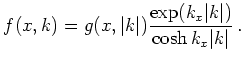
$$f(x,k) = g(x,\vert k\vert) \frac{\exp(k_x\vert k\vert)}{\cosh{k_x\vert k\vert}} .$$ (2.18)

This distribution has an isotropic symmetric part, but is not of the ``linear-isotropic'' type. Under the shifting assumption the distribution function $f$ is given by two ``1+1'' unknowns $g$ and $h$. Computationally this reduces the three-dimensional $k$-space to two one-dimensional distributions in $\vert k\vert$.

Further functional forms of the distribution function emerge, e.g., from the maximum entropy closure or from an expansion in Hermite polynomials. The choice of the functional form is necessary to describe the distribution function by a reduced set of moments within the moments method, see Section 2.2.