We use Dirichlet boundary conditions for
the even moments stemming from a ``cold'' Maxwellian distribution.
We also assume local charge neutrality at the boundaries,
that is, the carrier density ![]() is equal to the doping
is equal to the doping ![]() .
.
The equilibrium values
![]() are a
function of the lattice temperature
are a
function of the lattice temperature
![]() and for parabolic
band we obtain
([Gri02], page 17):
and for parabolic
band we obtain
([Gri02], page 17):
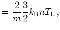 |
(2.49) | |
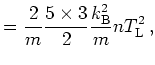 |
(2.50) | |
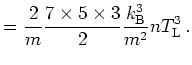 |
(2.51) |
![]()
![]()
![]()
![]() Previous: 2.2.3 Closure Problem
Up: 2.2 The Method of
Next: 2.3 Closure Relations for
Previous: 2.2.3 Closure Problem
Up: 2.2 The Method of
Next: 2.3 Closure Relations for