Previous: 6.1.1 Wave Mechanics
Up: 6.1.1 Wave Mechanics
Next: 6.1.1.2 Von Neumann Equation
Previous: 6.1.1 Wave Mechanics
Up: 6.1.1 Wave Mechanics
Next: 6.1.1.2 Von Neumann Equation
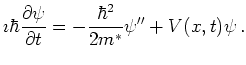
The time-dependent single-particle Schrödinger equation is
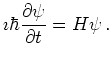 |
(6.1) |
Here  is the complex wave function.
The Hamiltonian operator
is the complex wave function.
The Hamiltonian operator  is a
Hermitian (self-adjoint) linear operator acting on the state space.
The Hamiltonian describes the total energy of the system.
is a
Hermitian (self-adjoint) linear operator acting on the state space.
The Hamiltonian describes the total energy of the system.
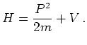
For a particle with
potential energy  the Hamiltonian is
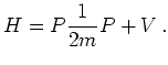
If the effective mass  is space dependent we choose
the operator ordering
is space dependent we choose
the operator ordering
to get a self-adjoint Hamiltonian.
In all our applications the effective mass is piecewise
constant.
Position and momentum operators obey the
canonical commutation relations
![$\displaystyle [ X^{i}, P^{j} ] = \imath \hbar \delta^{ij} .$](img315.png) |
(6.4) |
In one-dimensional position space
 the position
operator
the position
operator  is given by
 (i.e., multiplication of
  by ). The
momentum operator
by ). The
momentum operator  is then given by
 .
With this the transient Schrödinger equation for the electron wave function
on the real line
.
With this the transient Schrödinger equation for the electron wave function
on the real line
 reads (with constant mass)
 |
(6.5) |
In the so called time-independent case the wave
function is of the form
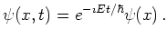 |
(6.6) |
As time progresses, the state vectors change only by a complex phase
and Schrödinger's equation becomes an eigenvalue equation for the
Hamiltonian ,
 |
(6.7) |
or with 6.2
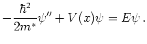 |
(6.8) |
The inner product in the Hilbert space determines the
probabilistic structure. Observables are represented by
self-adjoint operators.
The inner product
 of
two vectors is given by
of
two vectors is given by
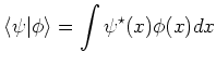 |
(6.9) |
where we used Dirac's ``bra-ket'' notation.
The eigenvectors of the position operator are denoted by
 , we write
  for the eigenvectors
of the momentum operator.
The wave functions and
for the eigenvectors
of the momentum operator.
The wave functions and  are then recovered as
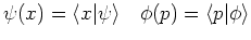 |
(6.10) |
for abstract wave vectors  ,
,  .
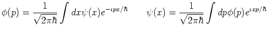
The relation beween space and momentum representation is
a Fourier transformation
Observables are repesented by self-adjoint operators.
In the Dirac notation the expectation value of an
observable
.
The relation beween space and momentum representation is
a Fourier transformation
Observables are repesented by self-adjoint operators.
In the Dirac notation the expectation value of an
observable  given in state is denoted by
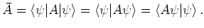 |
(6.11) |
Note that for non self-adjoint operators  the notation
 is ambiguous.
Previous: 6.1.1 Wave Mechanics
Up: 6.1.1 Wave Mechanics
Next: 6.1.1.2 Von Neumann Equation
R. Kosik: Numerical Challenges on the Road to NanoTCAD