Next: 4.3 Doping Characteristics
Up: 4. Doping and Trapping
Previous: 4.1 Introduction
For a disordered organic semiconductor system, we assume that
localized states are randomly distributed in both the energy and the
coordinate space, and that they form a discrete array of sites.
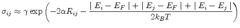
Conduction proceeds via hopping between these sites. In the case of low
electric field, the conductivity between site  and site
  can
be calculated as [17,44]
can
be calculated as [17,44]
 |
(4.1) |
where  and
and  are the energies at the sites
and , respectively,
are the energies at the sites
and , respectively,  is the Fermi-energy,
 is the distance between sites and , and
 is the Bohr radius of the localized wave function. The
first term
is the Bohr radius of the localized wave function. The
first term
 is a tunneling term, and the second one is a
thermal activation term (Boltzman term).
is a tunneling term, and the second one is a
thermal activation term (Boltzman term).
For organic semiconductors, the manifolds of both the lowest
unoccupied molecular orbitals (LUMO) and the highest occupied
molecular orbitals (HOMO) are characterized by random positional and
energetic disorder. Being embedded into a random medium, similarly,
dopant atoms and molecules are inevitably subjected to the
positional and energetic disorder, too. Since the HOMO level in most
organic semiconductors is deep and the gap separating LUMO and HOMO
states is wide, energies of donor and acceptor molecules are
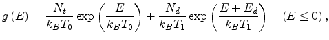
normally well below LUMO and above HOMO. So we assume
a double exponential density of states
 |
(4.2) |
where  and
and  are the concentrations of the intrinsic and
the dopant states, respectively,
are the concentrations of the intrinsic and
the dopant states, respectively,  and
and  are parameters
indicating the widths of the intrinsic and the dopant distributions,
respectively, and
are parameters
indicating the widths of the intrinsic and the dopant distributions,
respectively, and  is the Coulomb trap energy [92].
Vissenberg and Matters [43] pointed out that they
do not expect the results to be qualitatively different for a different choice
of
is the Coulomb trap energy [92].
Vissenberg and Matters [43] pointed out that they
do not expect the results to be qualitatively different for a different choice
of
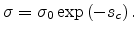
 , as long as
increases
strongly with
, as long as
increases
strongly with  . Therefore, we assume that transport takes
place in the tail of the exponential distribution.
. Therefore, we assume that transport takes
place in the tail of the exponential distribution.
The equilibrium distribution of carriers
 is determined by the Fermi-Dirac
distribution
is determined by the Fermi-Dirac
distribution
 as follows
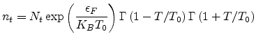
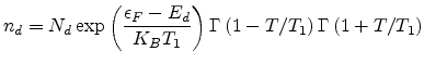
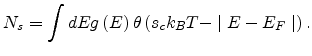
The Fermi-energy of this system is fixed by the equation for the carrier
concentration  ,
,
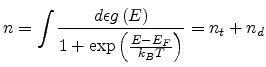 |
(4.3) |
where
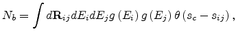
Here,  is the gamma function. According to the classical
percolation theory [17], the current will flow through
the bonds connecting the sites in a random Miller and Abrahams
network [9]. The conductivity of this system is
determined when the first infinite cluster occurs. At the onset of
percolation, the critical number
is the gamma function. According to the classical
percolation theory [17], the current will flow through
the bonds connecting the sites in a random Miller and Abrahams
network [9]. The conductivity of this system is
determined when the first infinite cluster occurs. At the onset of
percolation, the critical number  can be written as
 |
(4.4) |
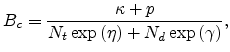
where  for a three-dimensional amorphous system,
  and
and
 are, respectively, the density of bonds and the density of
sites in this percolation system, which can be calculated by
[43,93,94].
are, respectively, the density of bonds and the density of
sites in this percolation system, which can be calculated by
[43,93,94].
 |
(4.5) |
 |
(4.6) |
Here
 denotes the distance vector between sites
and ,
denotes the distance vector between sites
and ,  is the unit step function, and
  is the
exponent of the conductance given by the relation [19]
is the
exponent of the conductance given by the relation [19]
 |
(4.7) |
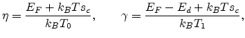
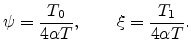
Substituting (4.2), (4.5) and (4.6) into (4.4), we obtain the expression,
 |
(4.8) |
where
Equation (4.8) has been obtained under the following conditions:
- the site positions are random,
- the energy barrier for the critical hop is large compared with
 ,
,
- and the carrier concentration is very low.
The exponent is obtained by a numerical solution of (4.8) and
the conductivity can be calculated using (4.7).
Next: 4.3 Doping Characteristics
Up: 4. Doping and Trapping
Previous: 4.1 Introduction
Ling Li: Charge Transport in Organic Semiconductor Materials and Devices
![$\displaystyle \rho\left(\epsilon\right)=
g\left(E\right)f\left(E\right)=\frac{g\left(E\right)}{1+
\exp\left[\left(E-E_F\right)/{k_BT}\right]}.$](img362.png)