2.1.1 Seebeck Effect

Figure 2.1: Thermocouple made of two metal rods.

Named after his discoverer, the Seebeck effect describes the occurrence of an electrical voltage induced by a temperature gradient. While the theoretical interpretation in Seebeck's pioneering paper [1] is surpassed by his general discovery by far, he also gave an overview of several material combinations usable in thermocouples as illustrated in Fig. 2.1.

Two rods of different materials are soldered together and the soldered points are held at the temperatures $\ensuremath{T_{\mathrm{H}}}$ and $\ensuremath{T_{\mathrm{C}}}$ , respectively maintaining a temperature difference $\Delta \ensuremath{T}$ and thus an according temperature gradient along the rods. On device level, the given temperature difference causes a certain voltage measured at the device's contacts

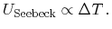$$\ensuremath{U_\ensuremath{\mathrm{Seebeck}}}\propto \Delta \ensuremath{T}\,.$$ (2.1)

In contrast to the frequently occurring idea in literature, that the Seebeck effect is based on the temperature dependence of the contact potential, the reason has to be looked for inside the device. Having a closer look on the microscopic description, the definition of the Seebeck coefficient is obtained by approaching infinitesimal small temperature differences. Then, a local potential gradient is caused by an according temperature gradient, which are connected by the temperature dependent Seebeck coefficient. Thus, the definition of the Seebeck coefficient reads

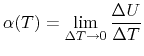$$\ensuremath{\alpha}(\ensuremath{T}) = \lim_{\Delta\ensuremath{T}\... ...%= \lim_{\Delta\vr \rightarrow 0} \frac{\Grad \potstatic \In \Delta \vr}{\Grad$$ (2.2)

The total voltage measured at the ends of one rod is given by the path integral along the rod as

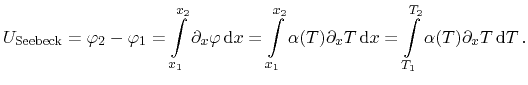$$U_\ensuremath{\mathrm{Seebeck}} = \ensuremath{\varphi}_2 - \ensur... ...h{T}) \ensuremath{\ensuremath{\partial_{x} \ensuremath{T}}} \d\ensuremath{T}\,.$$ (2.3)

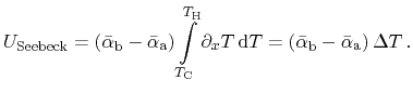
For the entire device, the path integral around the rods has to be evaluated. Beside the two constitutions of the single rods, the according contact potentials at the soldered points have to be added. However, the contact potentials cancel out each other and thus the voltage is given by

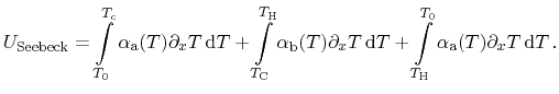$$U_\ensuremath{\mathrm{Seebeck}} = \int_{\ensuremath{T}_0}^{\ensur... ...h{T}) \ensuremath{\ensuremath{\partial_{x} \ensuremath{T}}} \d\ensuremath{T}\,.$$ (2.4)

By averaging the temperature dependent Seebeck coefficients along the rods, a combined coefficient for the material couple under given thermal conditions can be given as the difference of the single constituents of each rod

$$U_\ensuremath{\mathrm{Seebeck}} = \left( \bar{\ensuremath{\alpha}... ...r{\ensuremath{\alpha}}_\ensuremath{\mathrm{a}} \right) \Delta \ensuremath{T}\,.$$ (2.5)

Normally, two materials with Seebeck coefficients of different signs are chosen in order to gain an accordingly large voltage.

While the Seebeck coefficient of most metals is in the range of $1$ - $10\,\ensuremath{\mathrm{\mu V/K}}$ , values of $1\,\ensuremath{\mathrm{mV/K}}$ and more are obtained with semiconductors. Both metals with positive and negative Seebeck coefficients exist. The choice of according material combinations depends on the intention of use. For example in measurement applications, high total Seebeck coefficients are less important than a linear behavior in the desired temperature range. In semiconductors, the Seebeck coefficient can be varied by appropriate doping. While n-type semiconductors have negative Seebeck coefficients, the ones of p-type materials are positive. Quantitative values obtained in semiconductors can be obtained by analysis of carrier transport. Based on Boltzmann's equation, expressions for the coefficients are derived throughout Chapter 3.

M. Wagner: Simulation of Thermoelectric Devices