For the previous examination the Neumann boundary condition
(4.17) on
![]() is assumed to be zero (homogeneous Neumann boundary condition).
This subsection discusses which consequences are
drown from this assumption. Furthermore, it presents specific
models which require inhomogeneous (or non-zero) Neumann boundary
conditions to be assigned to define the field quantities or even
to preserve the physical consistence.
is assumed to be zero (homogeneous Neumann boundary condition).
This subsection discusses which consequences are
drown from this assumption. Furthermore, it presents specific
models which require inhomogeneous (or non-zero) Neumann boundary
conditions to be assigned to define the field quantities or even
to preserve the physical consistence.
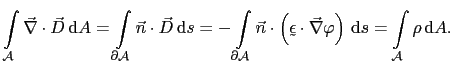
For the electrostatic case using (4.5), (4.8), and (4.10) it is written
However, the Neumann boundary condition cannot be arbitrarily chosen. For example, in the electrostatic case given by (4.11), Gauß's law (4.4) requires that the total electric flow through the boundaries must be equal to the electric charge inside the domain. For the two-dimensional case this is given by the expression
According to (3.18) the Neumann boundary condition
of (4.11) is (4.52).
In this case, if the surface electric charge in the entire
domain
![]() does not vanish,
physically it doesn't make sense to apply homogeneous Neumann
boundary conditions allover the entire boundary
does not vanish,
physically it doesn't make sense to apply homogeneous Neumann
boundary conditions allover the entire boundary
![]() .
.
In this work for the approximation of the inhomogeneous Neumann boundary condition an extension of the sum (4.13) with (4.22) from Section 4.1 is used
The coefficients are indexed in the following way:
The entire discretized domain contains ![]() nodes. The unknown coefficients
numbered from
nodes. The unknown coefficients
numbered from ![]() to
to ![]() correspond to the nodes which do not lie
on the Dirichlet boundary (the non-Dirichlet nodes). The known coefficients
numbered from
correspond to the nodes which do not lie
on the Dirichlet boundary (the non-Dirichlet nodes). The known coefficients
numbered from ![]() to
to ![]() (
(![]() ) correspond to the nodes on the
Dirichlet boundary (the Dirichlet nodes). The coefficients
) correspond to the nodes on the
Dirichlet boundary (the Dirichlet nodes). The coefficients ![]() from
(4.53) (
from
(4.53) (![]() ) must be obtained from
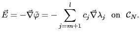
the Neumann boundary condition (4.17) on the Neumann
boundary
) must be obtained from
the Neumann boundary condition (4.17) on the Neumann
boundary
![]() . Thus, if
. Thus, if ![]() on the Neumann boundary
is given
on the Neumann boundary
is given
 |
(4.54) |
Now the Neumann boundary integral from (4.21) is given by
![$\displaystyle \int_{\mathcal{C}_N}\lambda_iD_n \mathrm{d}s = \sum_{j=m+1}^lc_j...
...vec{\nabla}\lambda_j\right) \mathrm{d}s = \sum_{j=m+1}^lc_jM_{ij}, i\in[1;n].$](img276.gif) |
(4.56) |
![\includegraphics[width=14cm,height=9.6cm]{figures/scalarfem2d/dissneumann.eps}](img279.gif) |
![\includegraphics[width=14cm,height=9.6cm]{figures/scalarfem2d/bigdissneumann.eps}](img280.gif) |
The acceptance of homogeneous Neumann boundary conditions is only
an approximation, which is not generally valid. This will be demonstrated by an
example. Let us consider the field generated by two electrodes with different
electrostatic potential applied. Let there be no other potential or charge density
distributions close to these electrodes to disturb this field. On the first electrode
0
V and on the second one ![]() V is impressed as shown in Fig. <4.5>, which is
given by Dirichlet boundary conditions for the
boundaries
V is impressed as shown in Fig. <4.5>, which is
given by Dirichlet boundary conditions for the
boundaries
![]() and
and
![]() between the simulation domain
between the simulation domain
![]() and the electrodes. The Laplace equation (4.12)
for the electric potential is solved in
and the electrodes. The Laplace equation (4.12)
for the electric potential is solved in
![]() . As usual, homogeneous Neumann
boundary conditions are set to the outer boundary
. As usual, homogeneous Neumann
boundary conditions are set to the outer boundary
![]() . This will not
influence the result, if the Neumann boundary is infinitely far away from the electrodes
and the corresponding Neumann boundary conditions can be neglected. In practice it is simulated with finite lengths
which normally results in simulation error. To demonstrate this behavior the same electrode
configuration is analyzed in a domain nine times larger than the domain in
Fig. <4.5>. Then the domain is cut off to the same region size as in
Fig. <4.5>. The corresponding electrostatic potential distribution is
shown by equipotential lines in Fig. <4.6>. This is compared to
the field in Fig. <4.5>. In contrast to Fig. <4.5> the field
on Fig. <4.6> corresponds to the expected one for the given configuration.
The homogeneous Neumann boundaries have distorted the simulation result in the small area
on Fig. <4.5>. Of coarse this is a systematic error, it gets smaller
with growing simulation domains.
For simulation of open regions the finite
element method can be combined with the boundary element
method [51,52,53]. This can also be performed
with the so called edge elements [54] introduced in
Chapter 5.
. This will not
influence the result, if the Neumann boundary is infinitely far away from the electrodes
and the corresponding Neumann boundary conditions can be neglected. In practice it is simulated with finite lengths
which normally results in simulation error. To demonstrate this behavior the same electrode
configuration is analyzed in a domain nine times larger than the domain in
Fig. <4.5>. Then the domain is cut off to the same region size as in
Fig. <4.5>. The corresponding electrostatic potential distribution is
shown by equipotential lines in Fig. <4.6>. This is compared to
the field in Fig. <4.5>. In contrast to Fig. <4.5> the field
on Fig. <4.6> corresponds to the expected one for the given configuration.
The homogeneous Neumann boundaries have distorted the simulation result in the small area
on Fig. <4.5>. Of coarse this is a systematic error, it gets smaller
with growing simulation domains.
For simulation of open regions the finite
element method can be combined with the boundary element
method [51,52,53]. This can also be performed
with the so called edge elements [54] introduced in
Chapter 5.