C.2.1 For the Scalar Function

Considering only the scalar functions $\psi$ the Neumann boundary term (5.31) is written

$$\int_{\mathcal{A}_{N2}}\lambda_i\vec{n}\cdot(\utilde{\mu}\cdot\ve... ..._i\vec{n}\cdot(\utilde{\mu}\cdot\vec{\nabla}\lambda_j) \mathrm{d}A = [D]\{c\}.$$ (C.27)

The matrix $[D]$ can be constructed by the element matrix $[D]^e$ with entries

$$D_{ij}^e = \mu\int_{\partial\mathcal{A}^e_k}\lambda^e_i \vec{n}_k\cdot\vec{\nabla}\lambda^e_j \mathrm{d}A, k\in[i;4], i\in[1;4], j\in[1;4].$$ (C.28)

$\mathcal{A}^e_k$ is the element face lying on the Neumann boundary $\mathcal{A}_{N2}$ and $\vec{n}_k$ is the corresponding normal vector pointing outwards. $\mu$ is assumed as constant scalar in each element. Again the element matrix is constructed for the four triangular faces (from $\mathcal{A}^e_1$ to $\mathcal{A}^e_4$ ) of the tetrahedron.

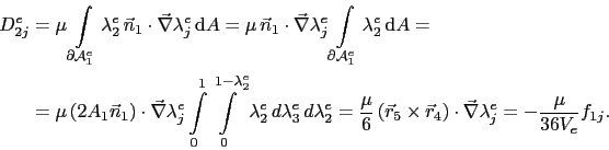
For $\mathcal{A}^e_1$ :

Since $\lambda^e_1$ is 0 on $\mathcal{A}^e_1$ $\Rightarrow$

$$D_{1j}^e = \mu\int_{\partial\mathcal{A}^e_1}\lambda^e_1 \vec{n}_1\cdot\vec{\nabla}\lambda^e_j \mathrm{d}A = 0.$$ (C.29)

For the second row the following expression is obtained

$$\begin{split}D_{2j}^e & = \mu\int_{\partial\mathcal{A}^e_1}\l... ...\vec{\nabla}\lambda^e_j = -\frac{\mu}{36V_e}f_{1j}. \end{split}$$ (C.30)

Analogously the entries of the next rows are calculated

$$D_{2j}^e = D_{3j}^e = D_{4j}^e = -\frac{\mu}{36V_e}f_{1j}.$$ (C.31)

The non-zero entries do not depend on the row index but on the face and column index. Consequently the non-zero rows are identical.

Similarly it is proceeded for the remaining element faces.

For $\mathcal{A}^e_2$ :

$$D_{2j}^e = 0, D_{1j}^e = D_{3j}^e = D_{4j}^e = -\frac{\mu}{36V_e}f_{2j}.$$ (C.32)

For $\mathcal{A}^e_3$ :

$$D_{3j}^e = 0, D_{1j}^e = D_{2j}^e = D_{4j}^e = -\frac{\mu}{36V_e}f_{3j}.$$ (C.33)

For $\mathcal{A}^e_4$ :

$$D_{4j}^e = 0, D_{1j}^e = D_{2j}^e = D_{3j}^e = -\frac{\mu}{36V_e}f_{4j}.$$ (C.34)