Based on a very simple model, Black [45,46,47] was the first to derive an expression for the time to failure of a metal line subjected to electromigration. He considered that the mean time to failure, ![]() , is inversely proportional to the rate of mass transport,
, is inversely proportional to the rate of mass transport, ![]() ,
,
It is interesting to note that the original equation (1.5) predicted a failure time proportional to the inverse square of the current density, even though mass transport due to electromigration had been shown to be linearly dependent on the current density [1]. This issue was discussed by several authors [48,49], however, the explanation for the square dependence was elucidated only several years later, when various theoretical works [50,51,52,53,54,55] considerably contributed to a better understanding of the electromigration behavior. An exponent close to 1 indicates that the lifetime is dominated by the void growth mechanisms, i.e. the time for a void to grow and lead to failure represents the major portion of the lifetime [51,52], while a value close to 2 indicates that void nucleation is the dominant phase of the electromigration lifetime [50,53,54,55].
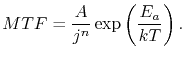
Since equation (1.6) connects the EM time to failure with the material transport mechanism via the activation energy parameter, and the current density dependence via the exponent ![]() . Thus, these parameters can be experimentally determined from the accelerated tests.
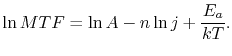
Taking the logarithm of (1.6) yields
. Thus, these parameters can be experimentally determined from the accelerated tests.
Taking the logarithm of (1.6) yields
![\includegraphics[width=0.45\linewidth]{chapter_introduction/Figures/Black_Ea.eps}](img98.png)
![\includegraphics[width=0.45\linewidth]{chapter_introduction/Figures/Black_n.eps}](img99.png)
|
This method of parameter extraction together with equation (1.6) has been used for lifetime estimation and extrapolation to operating conditions for 40 years now. However, in a recent publication Lloyd [56] discussed this application of the modified equation (1.6) and concluded that it may lead to significant errors in the lifetime extrapolation. These errors arise from the assumption that the fitting parameters ![]() ,
, ![]() , and
, and ![]() obtained under accelerated tests are also valid at real operating conditions, so that they can be directly applied for the lifetime extrapolation. As Lloyd [56] shows, the experimental determination of the above parameters does not consider important additional temperature and also pre-existing stress dependences, which yields incorrect parameter values and, consequently, lifetime extrapolation.
obtained under accelerated tests are also valid at real operating conditions, so that they can be directly applied for the lifetime extrapolation. As Lloyd [56] shows, the experimental determination of the above parameters does not consider important additional temperature and also pre-existing stress dependences, which yields incorrect parameter values and, consequently, lifetime extrapolation.
Black's equation provides useful insight into electromigration failure, however, it does not allow a thorough understanding of the underlying physics related to the electromigration behavior for which more sophisticated physically based models are required.