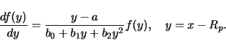
 |
(B9) |
with the coefficients
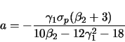 |
(B10) |
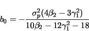 |
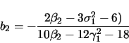
(B11) |
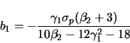 |
(B12) |
 |
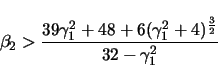
(B13) |
where Rp, ![]() ,
,
![]() ,
and
,
and ![]() are the projected
range, standard deviation, skewness and kurtosis, respectively.
The solution for the Pearson Type IV function is
are the projected
range, standard deviation, skewness and kurtosis, respectively.
The solution for the Pearson Type IV function is
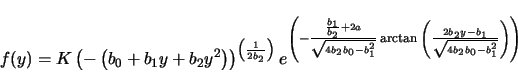 |
(B14) |
| (B15) |
 |
(B16) |
The maximum value is reached for x = Rp. The projected range Rp
is the average depth of the distribution. Skewness ![]() measures
the asymmetry of the distribution, a positive value places the peak
closer to the surface than the projected range. The kurtosis
measures
the asymmetry of the distribution, a positive value places the peak
closer to the surface than the projected range. The kurtosis ![]() describing the flatness of the top of the distribution.
describing the flatness of the top of the distribution.