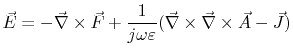
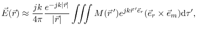
The electromagnetic field from electric and magnetic current sources in an unbounded
homogenous region can be expressed generally from
 |
(7.20) |
and
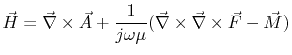 |
(7.21) |
with
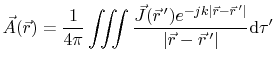 |
(7.22) |
and
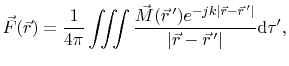 |
(7.23) |
where  is the electric field density,
  is the magnetic field density,
 is the magnetic vector potential,
  is the electric vector potential,
 is the vector to the magnetic and the electric current sources
in (7.22) and (7.23)
respectively,
is the vector to the magnetic and the electric current sources
in (7.22) and (7.23)
respectively,  is the permeability, and
 is the permittivity of the
homogenous region
is the permittivity of the
homogenous region  . This is described in more detail in [102].
With the angle  between the vectors
  and
, depicted in
Figure 7.2, the distance
and
, depicted in
Figure 7.2, the distance
 can be approximated with
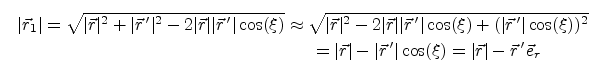 |
(7.24) |
in the far field, where  becomes large compared to
 . The
direction of is
. The
direction of is
 . For antennas with an active dimension
  ,
such as, for example, the length of a dipole, or the length of an aperture, the far field
region condition is
,
such as, for example, the length of a dipole, or the length of an aperture, the far field
region condition is
 |
(7.25) |
according to [104]. The wavelength in air is
 .
.
![\includegraphics[width=4cm,viewport=225 645 360
745,clip]{{pics/Far_Field_Approx.eps}}](img528.png)
Figure 7.2:
Angle between the vectors and
.
With (7.24) the electric vector
potential (7.23) in the far field region becomes
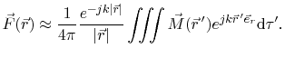 |
(7.26) |
The magnetic vector potential becomes
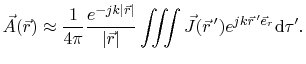 |
(7.27) |
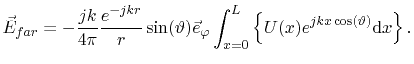
The radiation from the enclosure is mainly determined by the electric voltage
distribution at the slot [59]. From this voltage distribution an equivalent
magnetic source current on the slot is obtained as depicted in
Figure 7.3 for the calculation of the radiated electric far
field. With (7.20) the electric far field from magnetic current
sources
 |
(7.28) |
is applied on (7.26) to obtain the far field
approximation for the electric field density
 |
(7.29) |
according to [59], [69], where
 is the direction
of the magnetic current density
is the direction
of the magnetic current density
 .
.
![\includegraphics[width=12cm,viewport=80 510 510
745,clip]{{pics/Equivalent_Sources_Slot.eps}}](img535.png)
Figure 7.3:
Equivalent magnetic current sources at the enclosure slot for the derivation of
the radiated far field from the slot. This spherical angle definition was used, because
it enables simpler radiation field expressions.
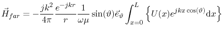
With the coordinate system definition and the equivalent magnetic current sources at the
slot depicted in Figure 7.3, (7.29)
for the electric far field becomes
 |
(7.30) |
The magnetic far field is described with
 |
(7.31) |
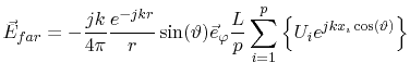
accordingly. With a declaration of  interface ports at the slot of the
enclosure, (7.30) is discretized to
interface ports at the slot of the
enclosure, (7.30) is discretized to
 |
(7.32) |
and (7.31) is discretized to
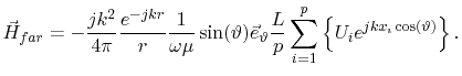 |
(7.33) |
 denote the voltages at the slot ports with the integer index
 ![$ i\in[1,p]$](img541.png) . The
far field condition (7.25) for the enclosure depicted in
Figure 7.3 becomes
. The
far field condition (7.25) for the enclosure depicted in
Figure 7.3 becomes
 |
(7.34) |
C. Poschalko: The Simulation of Emission from Printed Circuit Boards under a Metallic Cover