H.2 Recursive Algorithm to Calculate 
Following Appendix H.1, the algorithm to calculate the electron density
(diagonal elements of ) is discussed in terms of the DYSON equation for the
lesser and the left-connected GREEN's functions. The solution
to the matrix equation
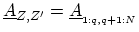
![$\displaystyle \left[ \begin{array}{cc} \ensuremath{{\underline{A}}}_{Z,Z} & \en...
...uremath{{\underline{G}}}^\mathrm{a}_{Z^\prime,Z^\prime} \end{array} \right] \ ,$](img1398.png) |
(H.12) |
can be written as
 |
(H.13) |
where
 and
and
 have been defined in (H.7)
and (H.8), and
have been defined in (H.7)
and (H.8), and
 and
and
 are readily identifiable from
(H.12). Using the relation
are readily identifiable from
(H.12). Using the relation
 , (H.13) can be written as
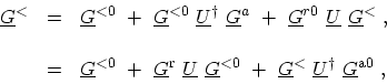 |
(H.14) |
where
 |
(H.15) |
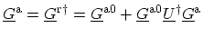
The left-connected lesser GREEN's function
 is defined by the first
  blocks of (H.2)
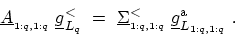 |
(H.16) |
 is defined in a manner identical to
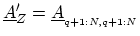
 except that the left-connected system
is comprised of the first
except that the left-connected system
is comprised of the first  blocks of (H.2).
In terms of (H.12), the equation governing
blocks of (H.2).
In terms of (H.12), the equation governing
 follows by setting
  and
and
 . Using the DYSON
equations for
. Using the DYSON
equations for
 and
,
and
,
 can be recursively obtained as [8]
 |
(H.17) |
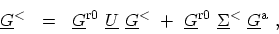
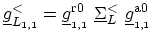
which can be written in a more intuitive form as
|
(H.18) |
where
 . Equation (H.18) has the physical meaning that
 has contributions due to four injection functions:
(i) an effective self-energy due to the left-connected structure that ends at
, which is represented by
has contributions due to four injection functions:
(i) an effective self-energy due to the left-connected structure that ends at
, which is represented by
 , (ii) the diagonal
self-energy component at grid point that enters (H.2), and
(iii) the two off-diagonal self-energy components involving grid points
and .
, (ii) the diagonal
self-energy component at grid point that enters (H.2), and
(iii) the two off-diagonal self-energy components involving grid points
and .
To express the full lesser GREEN's function in terms of the left-connected
GREEN's function, one can consider (H.12) such that
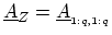 ,
,
 and
and
 . Noting that the only non-zero
block of
. Noting that the only non-zero
block of
 is
is
 and
using (H.14), one obtains
and
using (H.14), one obtains
 |
(H.19) |
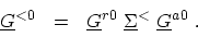
Using (H.14),
 can be written in terms
of
can be written in terms
of
 and other known GREEN's functions as
 |
(H.20) |
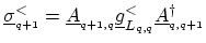
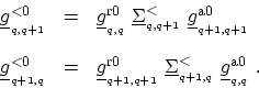
Substituting (H.20) in (H.19) and using (H.5), one obtains
![\begin{displaymath}\begin{array}{lll} \ensuremath{{\underline{G}}}^<_{_{q,q}}&=&...
...remath{{\underline{g}}}^{<0}_{_{q+1,q}} \right] \ , \end{array}\end{displaymath}](img1423.png) |
(H.21) |
where
 |
(H.22) |
The terms inside the square brackets of (H.21) are HERMITian conjugates
of each other. In view of the above equations, the algorithm to compute the
diagonal blocks of
is given by the following steps:
-
 ,
,
- For
 , (H.18) is computed,
- For
 , (H.21) and (H.22) are computed.
M. Pourfath: Numerical Study of Quantum Transport in Carbon Nanotube-Based Transistors