2.2.2.2 Interpretation Within the Relaxation Time Approximation

To understand the structure of a non-equilibrium state and the difference from an equilibrium state it is useful to consider the relaxation time approximation before the general theory. The relaxation time $\tau_{n}(\vec{r},\vec{k})$ is introduced in a way that the collision probability during the time interval $dt$ for an electron in band $n$ at phase space point $(\vec{r},\vec{k})$ is equal to $dt/\tau_{n}(\vec{r},\vec{k})$. In the relaxation time approximation it is inferred that some time after scattering has occurred the electron distribution does not depend on the non-equilibrium distribution just before the scattering. Additionally, if electrons have the equilibrium distribution with local temperature $T({\vec{r}})$:

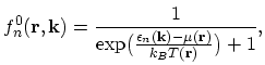$$f_{n}^{0}(\vec{r},\vec{k})=\frac{1}{\exp\bigl(\frac{\epsilon_{n}(\vec{k})-\mu(\vec{r})}{k_{B}T(\vec{r})}\bigr)+1},$$ (2.37)

the collisions do not affect the form of the distribution function. Therefore this approximation surmises that the information about the non-equilibrium state is completely lost due to the scattering processes^2.10 and that the thermodynamic equilibrium corresponding to a local temperature is maintained through the scattering. This totally specifies the distribution function of those electrons, which have been scattered near point $\vec{r}$ between $t$ and $t+dt$. This distribution function is denoted as $df_{n}(\vec{r},\vec{k},t)$. It cannot depend on the non-equilibrium distribution function $f_{n}(\vec{r},\vec{k},t)$. Thus $df_{n}(\vec{r},\vec{k},t)$ can be found assuming an arbitrary form of $f_{n}(\vec{r},\vec{k},t)$. This can be done for example using expression (2.37) for the local equilibrium taking into account the fact that the collisions do not change its form. During a time interval $dt$ an electron fraction $dt/\tau_{n}(\vec{r},\vec{k})$ in band $n$ with quasi-momentum $\hbar\vec{k}$ and coordinate $\vec{r}$ are scattered, changing their band number and quasi-momentum^2.11. The distribution function $f_{n}^{0}(\vec{r},\vec{k})$ cannot change which means that the distribution of those electrons which contribute to band $n$ with quasi-momentum $\hbar\vec{k}$ during the same time interval $dt$, must exactly offset for all the losses. This leads to the following expression:

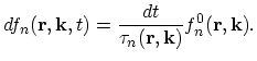$$df_{n}(\vec{r},\vec{k},t)=\frac{dt}{\tau_{n}(\vec{r},\vec{k})}f_{n}^{0}(\vec{r},\vec{k}).$$ (2.38)

This equation mathematically reflects the essence of the relaxation time approximation.

The number of electrons (2.36) in band $n$ at time $t$ in the phase space domain $d\vec{r}d\vec{k}$ can be alternatively found selecting electrons by the time of the last collision. Let $\vec{r}_{n}(t^{'})$ and $\vec{k}_{n}(t^{'})$ be the solutions of the semiclassical equations of motion, (2.7) and (2.14), for band $n$. Let this semiclassical trajectory pass through point $(\vec{r},\vec{k})$ at time $t^{'}=t$: $\vec{r}_{n}(t)=\vec{r}$, $\vec{k}_{n}(t)=\vec{k}$. If at time $t$ an electron was in the phase space domain $d\vec{r}d\vec{k}$ around $(\vec{r},\vec{k})$ and had been scattered during the time interval $[t^{'},t^{'}+dt^{'}]$, it must be scattered to the phase space domain $d\vec{r}^{'}d\vec{k}^{'}$ around $(\vec{r}_{n}(t^{'}),\vec{k}_{n}(t^{'}))$ because after time $t^{'}$ its trajectory is completely determined by the equations of motion. Using (2.38) the total number of electrons scattered from point $(\vec{r}_{n}(t^{'}),\vec{k}_{n}(t^{'}))$ into the phase space domain $d\vec{r}^{'}d\vec{k}^{'}$ during the time interval $[t^{'},t^{'}+dt^{'}]$ can be written as:

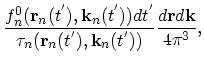$$\frac{f_{n}^{0}(\vec{r}_{n}(t^{'}),\vec{k}_{n}(t^{'}))dt^{'}}{\tau_{n}(\vec{r}_{n}(t^{'}),\vec{k}_{n}(t^{'}))}\frac{d\vec{r}d\vec{k}}{4\pi^{3}},$$ (2.39)

where the conservation law of the phase space volume has been used, that is, $d\vec{r}^{'}d\vec{k}^{'}=d\vec{r}d\vec{k}$. Some of these electrons are not scattered between time moments $t^{'}$ and $t$. Let the relative number of these electrons be $P_{n}(\vec{r},\vec{k},t,t^{'})$. Multiplying (2.39) by $P_{n}(\vec{r},\vec{k},t,t^{'})$ and summing over all possible values of $t^{'}$ gives the expression for $dN_{el}$:

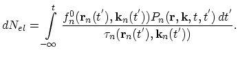$$dN_{el}=\int_{-\infty}^{t}\frac{f_{n}^{0}(\vec{r}_{n}(t^{'}),\vec... ...r},\vec{k},t,t^{'})\,dt^{'}} {\tau_{n}(\vec{r}_{n}(t^{'}),\vec{k}_{n}(t^{'}))}.$$ (2.40)

Comparison with (2.36) gives for the non-equilibrium distribution function:

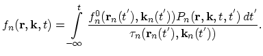$$f_{n}(\vec{r},\vec{k},t)=\int_{-\infty}^{t}\frac{f_{n}^{0}(\vec{r... ...r},\vec{k},t,t^{'})\,dt^{'}} {\tau_{n}(\vec{r}_{n}(t^{'}),\vec{k}_{n}(t^{'}))}.$$ (2.41)

The last expression clearly shows the structure of the non-equilibrium distribution function. The integrand includes the product of the total number of electrons scattered between $t^{'}$ and $t^{'}+dt^{'}$ and moving in such a way that they reach the phase space domain $d\vec{r}d\vec{k}$ at time $t$ assuming that no scattering events have occurred and the relative number of electrons which really reach the phase space domain $d\vec{r}d\vec{k}$. The contribution from all possible time moments is taken into account by the time integration.

S. Smirnov: