2. 6. 2 Discrete Solution Methods

A further step of complexity is the evaluation of quantities, namely functions which are defined on elements of at least one type of topological elements of the cell complex. For the following examples the cell complex considered is of dimension one, namely a graph.

In all of the considered models the modeling directly results in a discrete problem. The main reason for the use of a discrete model is that the continuous problem is cumbersome to describe and does not introduce any improvements on the accuracy of the results. Often discrete simulation models are used, if the exact physical behavior is not sufficiently known or if the physical behavior is too complicated to model.

In the following, simulation methods for electrical and mechanical circuits [69,70], methods for supply chain networks [71,72] are shown. Furthermore, a large variety of graph based problems can be investigated using the same topological framework, for instance neural networks [73], the simulation of telecommunication networks [74], or control networks [75].

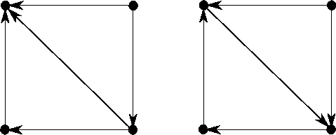
The underlying topological structure for all these simulation methods is a directed graph [76] (Fig. 2.9). Various implementations of graph data structures are currently available, mainly coupled with simulation tools for the branches mentioned above and only few of frameworks allow a data-structure independent implementation such as the Boost Graph Library [44].

Typical applications require the summation of all incident edges of a vertex with different weighting of ingoing and outgoing edges. In some cases, for instance for electrical or mechanical circuit simulation it is required to weight ingoing edges with the factor $+1$ and outgoing edges with the factor $-1$ or vice versa. In other cases, for instance supply chain simulation, only ingoing edges are considered, whereas outgoing edges are neglected.

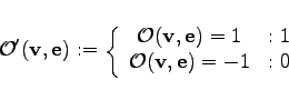
In terms of the topological framework of the GSSE, the direction information of the edges can be used in formulations by the orientation function. For the application of electrical networks this formulation is quite convenient. The first Kirchhoff Law can be written as follows

$$\sum_{VE}^{\underline{v}} \mathcal{O}(\bullet, \underline{v}) I = 0 \; .$$ (2.56)

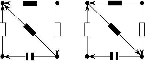
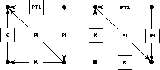
Many other simulation applications provide an inherent flow direction, for instance supply chain simulation. While for the simulation of electrical circuits the orientation of edges and vertices has to be defined arbitrarily (see Fig. 2.10), the orientation of edges and vertices in a supply chain has to be adapted to the special supply chain or a control network (see Fig. 2.11).

Figure 2.9: Directed graph with different orientations.
Figure 2.10: For the simulation of electrical circuits the orientation has to be given, but is not essential for the simulation.
Figure 2.11: For the simulation of control networks the orientation has been explicitly defined. Changes of the direction lead to a structurally different behavior.

In supply chain simulation, a processing facility, a machine, a transport lane, or a human is associated with a node or vertex. For a control network, a control element such as a control path or a controller associated to a vertex. If the output of one element associated with a vertex is required as input of another element, an edge incident with both vertices is introduced.

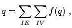
Typically, each element associated with a vertex fulfills a typical behavior, namely it takes its input as well as its internal state and processes one or more output values. In order to specify this behavior with the means shown in the previous section, the following formulation can be introduced

$$q = \sum_{VE}^{\underline{v}} \mathcal{O}'(\bullet, \underline{v}) \sum_{EV}^{\underline{e}} \mathcal{O}'(\bullet, \underline{e}) f(q) \; ,$$ (2.57)

where $q$ denotes the output quantity of a vertex. The processing of the input quantity is specified by the function $f$ . The modified orientation function $\mathcal{O}$ is defined as follows:

$$\mathcal{O}' (\mathbf{v}, \mathbf{e}):= \left\{ \begin{arr... ...cal{O} (\mathbf{v}, \mathbf{e}) = -1 & : 0 \end{array} \right.$$

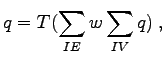
It can be seen easily that a number of output quantities is calculated and subsequently multiplied with zero. Even though this leads to a correct result, the performance of the calculation is unnecessarily worsened. For this reason a traversal method $IE$ can be used which only considers the vertices which are located on the ingoing edges of a given vertex. The traversal method $IV$ returns the source vertex of an edge. Using this formulation (2.57) can be simplified as follows:

$$q = \sum_{IE} \sum_{IV} f(q) \; ,$$ (2.58)

Such a method can be excellently applied to neural networks [77]. Each input is weighted with a predefined value $w$ defined on the respective connection edge and the sum of all weighted input quantities is formed. Afterwards a threshold function $T$ is applied to the weighted sum.

$$q = T(\sum_{IE} w \sum_{IV} q) \; ,$$ (2.59)

It can be seen that graph based discrete models can be easily written in the specification language proposed in the previous section. Graph based simulation methods can be formulated using the traversal methods introduced in this section.