3. 1. 1 Weak Formulation and Galerkin Schemes

The method is based on the notion of the weak formulation or weak solution, which is defined in the following manner: A function $u$ is a weak solution of a differential equation $\mathcal{L}(u) = 0$ within the domain $\mathcal{D}$ , iff for each function $w$ the following condition holds true:

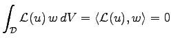
$$\int_\mathcal{D}\mathcal{L}(u) \, w \, dV = \langle \mathcal{L}(u) , w \rangle = 0$$ (3.1)

This condition can not hold true for arbitrary functions $w$ , because the underlying function space does not necessarily provide a weak solution. Consequently, one attempts to fulfill such a condition as well as possible. For this reason, a space $\mathcal{W}$ of special weighting functions $w_1 \ldots w_n$ is introduced, which is used to measure the deficiency of the numerical solution.

A widely used approach, which uses the shape functions as weighting functions is the Galerkin approach. It has been shown that such an approach has many advantages such as providing a symmetric equation system or system matrix.

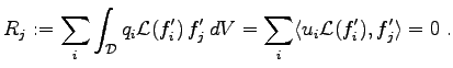
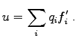
The typical formulation of a differential equation using the Galerkin finite element method is written as

$$R_j := \sum_i \int_\mathcal{D} q_i \mathcal{L}(f'_i) \, f'_j \, dV = \sum_i \langle u_i \mathcal{L}(f'_i) , f'_j \rangle = 0 \; .$$ (3.2)

The coefficients $q_i$ denote the weighting coefficients for the shape functions. The solution function can be written in terms of the shape functions in the following manner

$$u = \sum_i q_i f'_i \; .$$ (3.3)

It is assumed that the space of possible solution functions $\mathcal{F}'$ is derived from a given tesselation of the simulation domain as shown in Chapter 2. For the sake of simplicity linear shape functions are used, where single shape functions $f'$ collocate with vertices of the tesselation of the simulation domain.