3. 5 Final Considerations

The following remarks are common for all discretization schemes for differential equations and show their structural similarity, when written in the formalism according to Chapter 2.

Even if two or more solution variables are available on a topological element, the neighborhood is usually the same for all solution quantities, so that the considerations can be restricted to one solution quantity. In order to obtain the internal couplings within the system matrix, all quantities as well as their couplings have to be considered.

The first common feature which is fulfilled by all discretization schemes is that the solution quantity is located on topological elements. These elements are mostly vertices. For higher-order arrangements, especially for finite elements also other topological elements such as edges can be used.

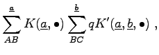
Each of the discussed discretization schemes establishes a topology defined by neighborhoods [64], where each element is assigned a neighborhood of elements. The neighborhood can be either directly retrieved from the underlying cell complex or derived from geometrical properties, e.g. for the finite difference method. In the following, the discretized differential operator is written as weighted sum of quantity values in the neighborhood of a topological element.

The process of obtaining neighboring elements is defined by two steps: firstly, the neighborhood $b$ of the initial element $a$ is retrieved by the traversal method $AB$ . Secondly, all elements $c$ of the neighborhood elements $b$ , on which relevant quantities are stored, are retrieved by the traversal methods $BC$ .

$$\sum_{AB}^{\underline{a}} K(\underline{a}, \bullet) \sum_{BC}^{\underline{b}} q K'(\underline{a}, \underline{b}, \bullet) \; ,$$ (3.63)

Here $AB$ and $BC$ denote the topological functions, of incident elements. It can be seen that for all discretization schemes coupling functions $K$ and $K'$ are required which yield coupling coefficients that finally are entered into the system matrix of the final equation system.

Discr. Scheme	Neighborhood	Neighb. Elem.
FEM (linear)	$\bigcup_{VC}$	$[\bigcup_{VC} \bigcup_{CV}]$
FVM (linear)	$\bigcup_{VE}$	$[\bigcup_{VE}\bigcup_{EV}]$
BEM (linear)	The cell complex	all vertices
	$\mathcal{B}$	$\bigcup{\mathcal{B}V}$
FDM (linear)	$\bigcup_{VN}$	$\bigcup_{VNV}$

For finite elements the neighborhood consists of the cells which are incident to the initial element. For finite volumes the neighborhood comprises all edges which are incident with the initial vertex. Boundary elements have a global neighborhood, i.e. each vertex is in the neighborhood of any other vertex. Finite differences do not explicitly give a neighborhood definition. It can be either derived from topological or from geometrical features.