Next: 5. 1. 2 GSSE Up: 5. 1 A Language for the Previous: 5. 1 A Language for the
For the sake of simplicity the treatment of the Laplace operator using the discretization schemes from Chapter 3 is discussed. For the first implementation only residual expressions are determined, however, the linearized expressions are shown in Setion 5.2. The expressions to be discretized are briefly reviewed:
 |
(5.1) | |
 |
(5.2) | |
 |
(5.3) | |
 |
(5.4) |
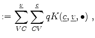
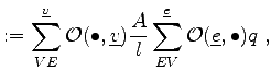
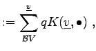
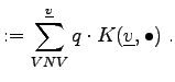
In the following implementation the coupling coefficients are determined locally with respect to geometric of physical quantities on the respective topological elements and are denoted as higher order functions K. For finite volumes the discretization formula is explicitly written.
 R_FEM = sum<VC>(_v)[sum<CV>(_c)[ q * K(_c, _v, _1) ]];
 R_FVM = sum<VE>(_v)[O(_1, _v)*A/d*sum<EV>(_e)[O(_e, _1) * q]];
 R_BEM = sum<CxV>(_v)[q * K(_v, _1)];
 R_FDM = sum<VNV>(_v)[q * K(_v, _1)];
It can be seen that the summation symbols ![]() are replaced by sum. The different kinds of traversal methods are written within angles, for instance the vertex on cell function
are replaced by sum. The different kinds of traversal methods are written within angles, for instance the vertex on cell function ![]() is referred to as <CV>. The named variables can be directly transformed into the DSEL by replacing
is referred to as <CV>. The named variables can be directly transformed into the DSEL by replacing
![]() by the similar and suggestive symbol v. This notation was taken from the Phoenix2 library [29] that intrinsically provides these symbols. Furthermore, the development of Phoenix2 was the main inspiration for choosing this special notation.
by the similar and suggestive symbol v. This notation was taken from the Phoenix2 library [29] that intrinsically provides these symbols. Furthermore, the development of Phoenix2 was the main inspiration for choosing this special notation.
The let-symbol is also taken from the Phoenix2 library and given the symbol ![]() within the functional calculus. Even though, the lambda function is also introduced in the Phoenix2 environment and can be directly introduced for creating higher order functions, its use was not required for the specification of discretized differential expressions. Furthermore, its use lead to a more complicated notation and drastically worsened the readability.
within the functional calculus. Even though, the lambda function is also introduced in the Phoenix2 environment and can be directly introduced for creating higher order functions, its use was not required for the specification of discretized differential expressions. Furthermore, its use lead to a more complicated notation and drastically worsened the readability.
Higher order functions such as the quantities as well as the coupling functions can be taken directly from the Phoenix2 library, where a simple interfacing to the underlying topological and quantity structures is possible.
Within the syntax of C++ an own language (DSEL) can be defined with which different expressions can be specified in a straight-forward manner. For the specification of these objects, object generators [88] as well as template expressions [89,90] are used.
Michael 2008-01-16