Next: 2. 2. 1 Functions and Discrete Representations Up: 2. Discrete Problems and Discretization Previous: 2. 1. 2 Errors of a Numerically Discrete Systems
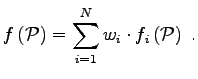
When these functions are stored in the computer, a function space comprising a finite number of basis vectors is introduced. Each function of this function space can be described as weighted sum of basis functions, ![]() where the weighting coefficients
where the weighting coefficients ![]() are stored as a vector-like data structure
are stored as a vector-like data structure
![]() , while the basis functions of the function space are assumed implicitly. Therefore, the function space covers all different functions which can be written as a linear combination of the following form
, while the basis functions of the function space are assumed implicitly. Therefore, the function space covers all different functions which can be written as a linear combination of the following form
 |
(2.5) |
The function space therefore represents the multitude of all possible functions which can be treated in the computer. From this point of view it is clear, that once the function and a special basis space are defined, only the coefficients need to be stored, whereas the shape of the basis functions is implicitly assumed.
In many cases the function space is defined in the following suggestive manner which is typical for finite difference schemes: Given a set of points
![]() , each of the base functions
, each of the base functions ![]() of the function space
of the function space
![]() is associated to one of the points
is associated to one of the points
![]() in a way that the following equation holds true, where
in a way that the following equation holds true, where
![]() denotes the Kronecker symbol.
denotes the Kronecker symbol.
| (2.6) |
For this reason, each weighting factor can be directly associated with the value of the function and the vector of these factors is understood as the set of points and their associated function values. Such an interpretation is very suggestive, because the rather abstract view on shape functions is replaced by direct function values, where the main problem is, however, that the information of the functional behavior between the points is lost. Differentiation, quadrature or the calculation of functionals is not possible from this point of view, because the information on the basis functions is ignored.
Finite element schemes [55] as well as boundary element schemes [56] define the underlying shape functions and then use form functionals, namely integrals, in order to determine the respective discrete dependences between the weighting factors of the functions. Even though the method can be written as an equation of weighting factors, the coupling of weighting coefficients strongly depends on the shape of the basis functions.
In contrast, finite difference schemes [57] and to some extent also finite volume schemes [33,58] do not explicitly define the underlying function space. They mainly rely on the discrete function values which are defined point-wise. Care has to be taken that for each discretization step the same interpolation scheme is used.