The indices  and
and  from (3.2) and (3.3) refer to the system matrix or to the numbering of the degrees of freedom in the function space
 . In this derivation, instead of indices, topological entities, in this simple case vertices, are used. Therefore, each function of the function space
can be directly associated with its corresponding vertex so that one can write
. In this derivation, instead of indices, topological entities, in this simple case vertices, are used. Therefore, each function of the function space
can be directly associated with its corresponding vertex so that one can write
 instead of
  , where
 is the vertex with index
.
In analogy, a function of the function space
is the vertex with index
.
In analogy, a function of the function space
 can be written as restriction of a function corresponding to a vertex
restricted on a cell
can be written as restriction of a function corresponding to a vertex
restricted on a cell
 , namely
 . It has to be assured that the vertex
and the cell
are incident in order to retrieve a valid, non-zero basis function of
.
As can be seen easily, these considerations can be used analogously for other topological entities on which quantities are stored. The substitution of the notation leads to the following formulation
. It has to be assured that the vertex
and the cell
are incident in order to retrieve a valid, non-zero basis function of
.
As can be seen easily, these considerations can be used analogously for other topological entities on which quantities are stored. The substitution of the notation leads to the following formulation
$](img231.png) |
(3.4) |
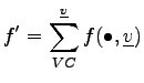
Next, the shape functions as well as the weighting functions, both from the function space
are written as functions of the function space
. This can only be applied, if the function space is derived from a tesselation of the underlying simulation domain and yields
 |
(3.5) |
with the resudial term  and
and
 |
(3.6) |
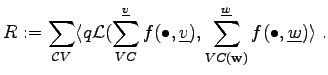
As the summands of the inner sums do not depend on the summation variables of the other summation, the sums can be written in the following manner:
$](img235.png) |
(3.7) |
Under the assumption that two functions of
, namely
 and
and
 can only yield a non-zero inner product,
has to be identical to
can only yield a non-zero inner product,
has to be identical to
 . Otherwise at least one of the functions is identically zero on the complete simulation domain. Furthermore, both of the vertices
and
. Otherwise at least one of the functions is identically zero on the complete simulation domain. Furthermore, both of the vertices
and
 have to be incident with the common cell
, because of the definition of the function space
. Figures 3.1 and 3.2 show the traversal mechanisms that have to be available for the implementation of finite element schemes.
have to be incident with the common cell
, because of the definition of the function space
. Figures 3.1 and 3.2 show the traversal mechanisms that have to be available for the implementation of finite element schemes.
Figure 3.1:
The finite element scheme applied to an unstructured cell complex.
|
|
Figure 3.2:
The finite element scheme applied to a structured cell complex.
|
|
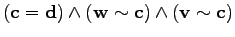 |
(3.8) |
Under the assumption of condition (3.8) the summation can be simplified to
![$\displaystyle R(\mathbf{w}) = [\sum_{VC}^{\underline{v}} \sum_{CV}^{\underline{...
..._{\underline{c}, \bullet} \rangle}_{K (\underline{c}, \underline{v}, \bullet)}]$](img242.png) |
(3.9) |
The quadrature of the respective shape functions can be performed in a straight forward manner. Moreover, different differential equations, quadrature methods shape functions, weighting functions quadrature methods and even inner products can be chosen without affecting the overall algebraic structure of the equation system. The specialization to a certain set of methods can be reduced to formulating a proper coefficient function  .
.
Michael
2008-01-16
![\includegraphics[width=10cm]{DRAWINGS/fem_topo.eps}](img239.png)
![\includegraphics[width=10cm]{DRAWINGS/fem_equi.eps}](img240.png)