For the discretization of the drift-diffusion semiconductor equations the flux terms have to be considered. In a divergence formulation, the stationary drift-diffusion semiconductor equations [33] can be specified as
The associated flux terms
 ,
,
 and
and
 are usually defined in the following way
The solution functions are the carrier concentrations  and
and  and the electrostatic potential
  . Here,
 denotes the permittivity coefficient,
  denotes the mobility of the carriers,
  denotes the generation/recombination rate for the carriers, and
  denotes the net doping.
For the sake of simplicity, only the electron carrier density is considered. By replacing the respective signs, the calculations can also be performed for the hole continuity equation. However, the final result will also be given for holes.
First, the Poisson equation is discretized in analogy to the Laplace equation. The respective flux relation for the dielectric displacement can be written in as expression evaluated on an edge. For this evaluation, the function values of the potential are evaluated on the bounding vertices of the edge.
The application of the finite volume scheme on this flux operator yields the following discretization scheme. In addition, the right hand side is approximated by multiplying with the cell volume.
$](img340.png) |
(3.41) |
It is reasonable to associate the flux related quantity
with the edge so as to obtain a straight-forward formulation. If the dependence of the electric field and displacement is modeled in a non-linear manner, all coefficients which are related to the determination of the displacement from the field strength can be associated to the respective edge.
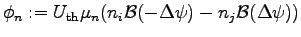
Secondly, the continuity equation for electrons is considered. In contrast to the linear interpolation for the potential along a connecting edge of two vertices, the carrier concentration is interpolated using the Scharfetter-Gummel discretization [3]. The interpolation does hereby depend on the potential which is given on the boundary nodes of the respective edge.
Even though the Scharfetter Gummel discretization was usually defined for one-dimensional discretization, many simulation tools [59] use the interpolation along the edges for two-dimensional or three-dimensional simulation. In its original formulation the Scharfetter Gummel discretization of the electron flux can be written as
 |
(3.42) |
where  and
and  denote the carrier concentration in the boundary vertices indiced by
  and
and  .
.
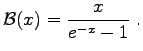
 denotes the Bernoulli function
 |
(3.43) |
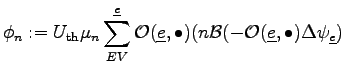
In analogy to the permittivity coefficient, the mobility for carriers can be stored on the edges. Furthermore, coefficients describing the dependence of the mobility on carrier concentration and potential can be associated with the respective edge. In the following model,
 is assumed to be a constant or a model-dependent global variable which is not associated to topological elements.
 |
(3.44) |
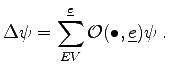
The potential dependent term in the Scharfetter Gummel scheme
 denotes the potential difference between two bounding vertices of an edge,
 . Based on the edge the formulation can be written in the following manner:
 |
(3.45) |
Michael
2008-01-16
![$\displaystyle = [\varepsilon \cdot \sum_{EV}^{\underline{e}} \mathcal{O}(\underline{e}, \bullet) \psi]$](img339.png)