4. 2. 2 Applications on Finite Element Schemes

For finite elements the element-wise assembly is carried out by the quadrature of all integral expressions which are related to a common cell $\mathbf{c}$ . In the case of a triangular cell which contains three vertex values, nine integrals have to be calculated. When Galerkin schemes are used, the calculation can be reduced to six integrals, because of the symmetry of the local matrix. The matrix can be written in the following manner, where the vertices of the cell $\mathbf{c}$ are denoted as $\mathbf{v}_1$ , $\mathbf{v}_2$ and $\mathbf{v}_3$

$$\mathbf{K} = \left[ \begin{array}{c c c} K(\mathbf{v}_1, \mathbf{... ... \mathbf{v}_2) & K(\mathbf{v}_3, \mathbf{c}, \mathbf{v}_3) \end{array}\right]$$

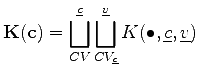
In the notation according to Chapter 2, such a local element matrix can be assembled using the vectorization command $\bigsqcup$ in order to retrieve a matrix.

$$\mathbf{K}(\mathbf{c}) = \bigsqcup_{CV}^{\underline{c}} \bigsqcup_{CV_{\underline{c}}}^{\underline{v}} K(\bullet, \underline{c}, \underline{v})$$ (4.37)

Figure 4.5: Element-wise assembly. For the finite element method all coupling coefficients which are determined by integrals over a common cell $\mathbf{c}$ are assembled together.

As can be seen in Figure 4.5, the matrix is assembled by local element matrices which are added to the system matrix. With the formalism introduced in Chapter 2 the local system matrix can be formulated.