


Next: 6. Examples
Up: 5. The Solver Module
Previous: 5.5 Practical Evaluation of
The performance evaluation resulted in conclusions which solver system has to
be activated for which kind of simulation. As already stated above, the solver
system as a core module of a simulator is frequently regarded as a black box
obliged to deliver the ``correct'' results in a ``short'' time. Hence, the
conclusions can be used to implement an automatic solver selection in the
simulator. Depending on the simulation mode, for example mixed-mode, the
best-suited solver system is chosen, which results in an overall speed-up of
the simulator without any user interaction.
Whereas the concept and objective of the performance evaluation has been proven
to be worthful and promising, the executive part can be improved in order to
obtain more specific and validated data:
- The extension of the simulation examples set: the current set can be
extended by examples of the same type and by new simulation modes, for
example by the six moments transport model. Since the benchmark program is
extensible and fully automated, there is virtually no limit besides a
reasonable run-time of the complete benchmark. Whereas the original set of
examples has pursued the idea of orthogonal examples, which means that they
are widely independent from each other, more examples of the same type would
yield more significant averages.
- A more differentiating grouping of the results: the existing
three groups can be split into more subgroups. For example the
three-dimensional examples can be grouped in various dimension ranges,
which would allow to assess the choice of iterative and direct solvers more
accurately. In addition, the transport models shall form separate
groups. Keeping the objective of an automatic solver selection in mind, the
grouping can be based on any parameter known in advance, for example
simulation mode, dimension, transport model etc.
- Taking the memory consumption into account: As discussed also in
[5] for harmonic balance simulations, the selection can be
additionally based on the respective amount of required memory compared with
the memory available.
If costly simulations are considered, the required
memory can become an interesting criterion. Since a simulator is able
to detect the host type and the amount of available memory, this criterion
can also be part of an automatic solver selection.
- The data conditioning and visualization of all results: in
addition to the grouping, averaging, and scaling of the results, a more
sophisticated profiling of the various solvers can be given.
Basically, the results are obtained by running a solver on a set of  examples and measuring interesting data, for example the simulation time. In
[79], a performance profile is used to evaluate and compare the
performance of various solvers. This profile is defined as follows: for an
example
examples and measuring interesting data, for example the simulation time. In
[79], a performance profile is used to evaluate and compare the
performance of various solvers. This profile is defined as follows: for an
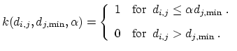
example  the solver
  yields the data
  . Since for all examples the
performance of the solver shall be compared with that of the best solver,
. Since for all examples the
performance of the solver shall be compared with that of the best solver,
 is defined as the minimum data of all solvers for the example .
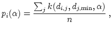
Depending on an
is defined as the minimum data of all solvers for the example .
Depending on an
 the performance profile of solver is given
by
the performance profile of solver is given
by
 :
:
 with with |
(5.3) |
 |
(5.4) |
The performance profile gives the fraction of examples for which solver is
within a factor of  of the best. Thus,
  is the fraction for
which solver gave the best results.
is the fraction for
which solver gave the best results.  is the fraction for which
solver is within a factor of 2 of the best. Finally,
is the fraction for which
solver is within a factor of 2 of the best. Finally,
 is the
fraction for which solver could be successfully employed at all. The last
value is particularly interesting, since it is inevitable that the benchmark
takes failures explicitly into account.
is the
fraction for which solver could be successfully employed at all. The last
value is particularly interesting, since it is inevitable that the benchmark
takes failures explicitly into account.
Next: 6. Examples
Up: 5. The Solver Module
Previous: 5.5 Practical Evaluation of
S. Wagner: Small-Signal Device and Circuit Simulation