4.3.1.4 Model Definition

To define a new model, the user must specify the model name and its solution vector as shown in the example:

MODEL <modelname> = [<Q1>,<Q2>,...,<Qn>];  # solution vector with 
                                           # quantities Q1,Q2 to Qn 
{
   <discretized PDEs>
   residuum = [f1(<Q1>),f2(<Q2>),...,fn(<Qn>)];  # the resulting
                                                 # residual function
   jacobian = D([<Q1>,<Q2>,...,<Qn>],residuum);  # the Jacobian matrix 
                                                 # automatically 
                                                 # calculated with the 
                                                 # derive operator
}

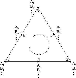
This environment automatically defines the three scalar time variables (t₀,t_{t - 1},t_{t - 2}) and defines n quantity vectors (Q₁,Q₂,...,Q_n) with three different time dependencies. For simpler understanding consider a model on a triangular mesh using quadratic shape functions for a finite element discretization (Fig. 4.4). In this case each quantity is represented as a vector of dimension 1x6, where the index of the vector refers to the value of the quantity on the belonging point of the triangle. Actually, the size of the vectors depends on the number of discretization points of an element and is automatically detected by the simulation system at run time. Furthermore, AMI creates coordinate vector variables with the same semantics as for the quantity variables. These vector variables are predefined as X,Y and Z and can be treated for discretization purposes in the same manner as any defined variable. In case of moving grid problems (e.g. oxidation, mechanical deformation), where the geometry is deformed and the coordinates itself are unknown quantities, the solution vector must include the variables named X,Y and Z which is a means to define time dependent coordinate values and an implicit definition of moving grid problems.

Figure 4.4: Discretized solution vectors on a triangular grid element

# implicit quantity vector
# definition of A,B, ...
# depending on the number
# of element nodes

During run time the values of the coordinates and quantities are transmitted to the AMI layer that replaces the variables with the values and evaluates the model. The results (normally residual and its derivative, the Jacobian matrix) are assembled into a global stiffness matrix.