3.1 Theory
The main idea of the SHE method is to expand the distribution function fν(x,k,t) into spherical
harmonics (SH)
Y l,m(θ,φ) = 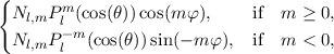 | | (3.1) |
where Plm(x) are the associated Legendre polynomials, l ≥ 0 is the order, m is the sub-order index
bounded by -l ≤ m ≤ l, and Nl,m are normalization factors given by
Nl,m = 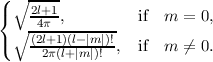 | | |
The spherical harmonics form an orthonormal basis since
 ≡∮Y l,mY l′,m′ ≡∮Y l,mY l′,m′ ≡dΩ = δl,l′δm,m′, ≡dΩ = δl,l′δm,m′, | | |
where the Kronecker delta δa,b = 1 if and only if a = b, else it equates to zero. Additionally, the
shorthands ∮
and dΩ have been introduced. With the above definition of the spherical harmonics, the
truncated expansion of the distribution function f(x,k,t) is
| f(x,k,t) ≃∑
l=0L ∑
m=-llf
l,m(x,ϵ,t)Y l,m(θ,φ), | | (3.2) |
where the order l is bounded by the maximum expansion order (l < L), ϵ is the energy, θ and φ are
the spherical angles of the spherical harmonics Y l,m [64, 66, 59, 47]. Additionally, the
expansion of the distribution function in spherical harmonics on equi-energy surfaces implicitly
assumes a bijective mapping E(k) (cf. Chapter 2) between energy and wave vector. An
exhaustive treatment of the derivation of the BTE expanded in spherical harmonics can be
found in [47]. For the sake of clarity the derivation will be briefly summarized in here. In
order to avoid notational clutter, the band index ν will be dropped in this chapter entirely,
since the projection on spherical harmonics does not change anything regarding the band
index. With this, any physical quantity X can be expanded into SH on equi-energy surfaces
using
| X ≃∑
l=0L ∑
m=-llX
l,m(ϵ)Y l,m(θ,φ). | | (3.3) |
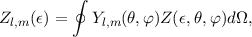
The expansion coefficients for any quantity X on equi-energy surfaces are then found as
[67, 47]
| Xl,m | =  ∫ ∫
 Y l,m(θ(k),φ(k))X(x,k)δ(ϵ - E(k))d3k Y l,m(θ(k),φ(k))X(x,k)δ(ϵ - E(k))d3k | |
|
| = ∮
Y l,m(θ,φ)X(x,k(ϵ,θ,φ))Z(ϵ,θ,φ)dΩ, | (3.4) |
where δ is the Dirac delta. Projecting the distribution function f(x,k,t) using Equation (3.4) one
obtains the expansion coefficients fl,m as
| fl,m | =  ∫
Y l,m(θ(k),φ(k))f(x,k,t)δ(ϵ - E(k))d3k ∫
Y l,m(θ(k),φ(k))f(x,k,t)δ(ϵ - E(k))d3k | |
|
| = ∮
Y l,m(θ,φ)f(x,k(ϵ,θ,φ),t)Z(ϵ,θ,φ)dΩ, | (3.5) |
The generalized density of states Z(ϵ,θ,φ) for a single spin direction in the absence of magnetic fields
transformed to spherical coordinates is
Z(ϵ,θ,φ) =   . . | | (3.6) |
Due to the integration over the spherical angles the generalized density of states differs by a factor of
4π from the conventional density of states.
3.1.1 Expansion of the Free-Streaming Operator
In order to obtain a set of equations for the expansion coefficients up to order L, the BTE is
multiplied by the generalized density of states (cf. Equation (3.6)), Y l,m, and afterwards integrated
over the unit sphere. Hence, a spherical harmonics expansion of the BTE,
 | (3.7) |
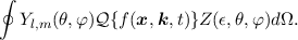
to find the unknown expansion coefficients fl,m, reads
| ∮
Y l,m(θ,φ){BTE}Z(ϵ,θ,φ)dΩ. | | (3.8) |
More precisely,
| ∫
Y l,mδtf(x,k,t)δ(ϵ - E(k))d3k | |
|
| + ∫
Y l,m {f(x,k,t)}δ(ϵ - E(k))d3k {f(x,k,t)}δ(ϵ - E(k))d3k | (3.9)
|
| = ∫
Y l,m( {f(x,k,t)}- Γ)δ(ϵ - E(k))d3k, {f(x,k,t)}- Γ)δ(ϵ - E(k))d3k, | | |
where the recombination term Γ will be treated separatly in Section 3.5 and the time-dependent term
will be discussed in detail later. In a second step the expansion 3.2 as well as a spherical
harmonics expansion for the density of states are used in Equation (3.9) in order to find
the equations per spatial location x, energy ϵ, order l and m [67, 47]. Assuming that
Z(ϵ,θ,φ) = Z(ϵ) the equations for the expansion coefficients fullfilling the BTE read term by term
[67],
| ∂tf(x,k,t) | ⇒ ∂t ∮
Y l,mf(x,ϵ,t)Z(ϵ)dΩ, | (3.10)
|
| vν
g(x,k)⋅∇xf(x,k,t) | ⇒∇x⋅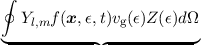 jl,m(x,ϵ,t), jl,m(x,ϵ,t), | (3.11)
|
| F(x,t)⋅∇kf(x,k,t) | ⇒ F(x,t)⋅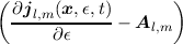 , , | (3.12)
|
| Al,m | = ∮
 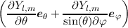 fZ(ϵ)dΩ, fZ(ϵ)dΩ, | (3.13) |
where eθ and eφ are the unit vectors in the space spanned by the spherical harmonics. Whilst the
time-dependent term can be projected in a straight-forward manner, the free streaming operator
{f(x,k,t)} is commonly split into two separate contributions. These two contributions are then also
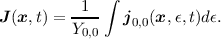
separatly transformed. The first contribution (cf. Equation (3.12)) is often referred to as the diffusion
term, since it can be expressed as the divergence of a generalized current density jl,m(x,ϵ,t). The
definition of the generalized current density is very convenient since the current density of charge
carriers is obtained by
 | (3.14) |
The second contribution to the transformed free streaming operator is referred to as the drift term,
since this term contains the force F and no spatial derivative.
3.1.2 Expansion of the Scattering-Streaming Operator
The scattering operator {f(x,k,t)} is split into an in-scattering and an out-scattering
term,
 | (3.15) |
Each term is then transformed to spherical coordinates on equi-energy surfaces by
 | (3.16) |
Utilizing the low-density approximation [68] for the scattering operators in Equation (2.30) the
transformation simplifies to
| in{f(x,k,t)} | ⇒∮
Y l,mZ(ϵ)∮
σ(k(ϵ′,θ′,φ′),k(ϵ,θ,φ))f(x,ϵ′,t)Z(ϵ′)dΩ′dΩ, | (3.17)
|
| out{f(x,k,t)} | ⇒∮
Y l,mZ(ϵ)∮
σ(k(ϵ,θ,φ),k(ϵ′,θ′,φ′))f(x,ϵ,t)Z(ϵ′)dΩ′dΩ, | (3.18) |
where it was assumed that the charge carrier is scattered from energy ϵ′ to ϵ. The physics of the
scattering process itself are summarized in the function σ. In this framework, the scattering process is
considered to be elastic if ϵ′ = ϵ, else it is an inelastic process. If the scattering operators are assumed
to be velocity randomizing [68], i.e. the projected rates σ do not depend on the angles, the projection
can be simplified further to yield
| in{f(x,k,t)} | ⇒ σ(ϵ′,ϵ)∮
Y l,mZ(ϵ)∮
f(x,ϵ′,t)Z(ϵ′)dΩ′dΩ, | (3.19)
|
| out{f(x,k,t)} | ⇒ σ(ϵ,ϵ′)∮
Y l,mZ(ϵ)∮
f(x,ϵ,t)Z(ϵ′)dΩ′dΩ. | (3.20) |
This can be considerably simplified by inserting the projection of the generalized density of
states,
 | (3.21) |
into Equation (3.22). After a few algebraic operations the scattering operators finally can be reduced
to read,
| in{f(x,k,t)} | ⇒ σ(ϵ′,ϵ)∮
Y l,mZ(ϵ)∮
f(x,ϵ′,t)Z(ϵ′)dΩ′dΩ | |
|
| =  σ(ϵ′,ϵ)Zl,m(ϵ)Z(ϵ′)fl′,m′(ϵ′,t)δ0,l′δ0,m′ = l′,m′,l,min, σ(ϵ′,ϵ)Zl,m(ϵ)Z(ϵ′)fl′,m′(ϵ′,t)δ0,l′δ0,m′ = l′,m′,l,min, | (3.22)
|
| out{f(x,k,t)} | ⇒ σ(ϵ,ϵ′)∮
Y l,mZ(ϵ)∮
f(x,ϵ,t)Z(ϵ′)dΩ′dΩ | |
|
| =  σ(ϵ′,ϵ)Z0,0(ϵ′)Z(ϵ)fl′,m′(ϵ,t)δl,l′δm,m′ = l′,m′,l,mout. σ(ϵ′,ϵ)Z0,0(ϵ′)Z(ϵ)fl′,m′(ϵ,t)δl,l′δm,m′ = l′,m′,l,mout. | (3.23) |