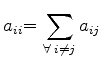
In the particular case of MOS structures, a point distribution with low point density along the channel and high point density towards the bulk seems feasible. Nevertheless, to fulfill the Delaunay criterion, the grid generator sometimes has to insert additional grid points. Therefore, a method for point insertion which does not violate the Delaunay criterion must be found.
For ortho-product grids, the aspect ratio of the cuboids can be varied arbitrarily. As mentioned before, an ortho grid can be transformed easily to a tetrahedral grid by splitting each cuboid into five or six tetrahedrons. The Delaunay criterion will never be violated, since all resulting tetrahedrons have the same outer-sphere and neighboring grid points can never lie within. A pleasant side effect of this method is that the coupling areas of the tetrahedrons inside the original parallelepiped will become zero, the resulting equation system will have fewer off-diagonal entries and the assembled equation system will be the same as the one obtained from the original ortho grid.
However, this approach is difficult when cuboids have to be fitted along geometry lines that are not in the same direction as the edges of the cuboids (refer Section 2.1). For maintaining the accuracy, the number of cuboids and, therefore, also the number of grid points will increase rapidly. In this case, the general use of tetrahedral grids is required. There are fewer geometry related limitations and a Delaunay grid can be found in most cases. But even an enhancement of the grid density will cause the tetrahedrons to become nearly equilateral (see Figure 5.5(b)) and a directional dependent grid density cannot be tuned arbitrarily. In the method developed here, the advantages of ortho and tetrahedral grids are combined.
The basic idea of the newly developed method can be explained by considering a nearly cuboidal capacitor with two electrodes.
The electric field outside the capacitor is neglected by assuming a high-k dielectric with a permittivity
![]() much higher than the vacuum permittivity. A sketch of such a capacitor is shown in Figure 5.6.
much higher than the vacuum permittivity. A sketch of such a capacitor is shown in Figure 5.6.
After applying a voltage between the electrodes, the equipotential lines and the field lines can be evaluated. The field lines are orthogonal to the potential lines. Additionally, either the equipotential or field lines are boundary-conform or orthogonal to the boundaries of the capacitor. If the spacing of selected potential and field lines of the capacitor is sufficiently small, two potential and two field lines lying next to each other approximately form rectangles, as shown in the figure. The spacing between the selected field and potential lines can be varied independently. To create a grid suitable for device simulation, these rectangles must be split into triangles by a mesh generator.
This method can be used for creating a set of grid points in a given domain. Four points at the boundary of this domain are placed at the corners of the capacitor. Between the corners, the upper and lower electrodes are located. After the evaluation of the field distribution, the grid points can be set at arbitrary intersections of the equipotential lines and field lines.
The field lines are not evaluated directly. Rather, they are evaluated by a duality, which can be applied if the following prerequisites are satisfied:
After applying a voltage between the electrodes, the electric potential distribution (
![]() ) inside the capacitor can be calculated and the equipotential lines (
) inside the capacitor can be calculated and the equipotential lines (
![]() ) can be evaluated.
) can be evaluated.
The field lines are evaluated via a duality in the specified way:
The dual electric field (
![]() ) and its associated equipotential lines (
) and its associated equipotential lines (
![]() ) are calculated.
) are calculated.
Now each point ![]() inside the capacitor can be represented by its potential representation
inside the capacitor can be represented by its potential representation
![]() .
.
In the two-dimensional case, there are four electrodes at the boundary of the capacitor -- two opposite electrodes of the original capacitor and the remaining two opposite boundaries as the electrodes for the dual capacitor. The extension of this method to three dimensions is as:
Such a capacitor can be seen in Figure 5.7.
The original capacitor delivers the field distribution
![]() with the equipotential surfaces
with the equipotential surfaces
![]() .
.
The electric field
![]() and its electric potential
and its electric potential ![]() , and as a consequence of this three-dimensional expansion, the electric field
, and as a consequence of this three-dimensional expansion, the electric field
![]() and the potential
and the potential ![]() , are derived as the resulting field inside a capacitor of the following shape:
, are derived as the resulting field inside a capacitor of the following shape:
With this new placement of the electrodes, the electric potential
![]() can be derived. By an additional replacement of the remaining two ``sides'' by electrodes and all others as insulator surfaces, the third potential
can be derived. By an additional replacement of the remaining two ``sides'' by electrodes and all others as insulator surfaces, the third potential
![]() can be calculated.
can be calculated.
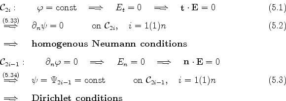
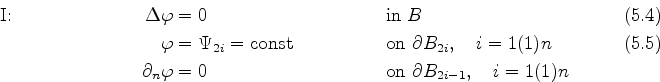
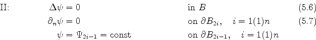
Inside the capacitor, the Laplace equation has to be solved (as shown in Section 3.1). The boundary conditions are
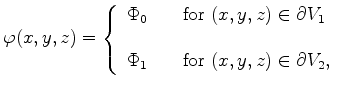 |
(5.16) |
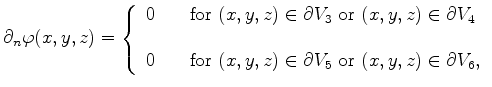 |
(5.17) |
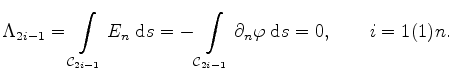
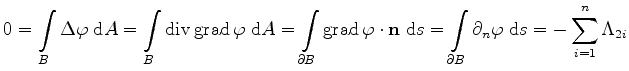
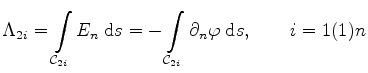
It can be seen that the elements defined by two appropriate equipotential lines of ![]() ,
, ![]() , and
, and ![]() are spanning the desired cuboids for the tetrahedrization. The different electrode placements with their assigned field distribution are illustrated in Figure 5.8 (original distribution), 5.9 (first electrode-replacement), and 5.10 (second electrode-replacement).
Resulting equipotential surfaces of all three field calculations are shown in Figure 5.11.
The full set of differential equations (assuming constant permittivity) with their assigned boundary conditions can be seen in Table 5.1.
are spanning the desired cuboids for the tetrahedrization. The different electrode placements with their assigned field distribution are illustrated in Figure 5.8 (original distribution), 5.9 (first electrode-replacement), and 5.10 (second electrode-replacement).
Resulting equipotential surfaces of all three field calculations are shown in Figure 5.11.
The full set of differential equations (assuming constant permittivity) with their assigned boundary conditions can be seen in Table 5.1.
![\includegraphics[width=13cm]{picsconveps/ticks}](img490.png)
|
In general, a realistic devices are more complex than such capacitors and therefore, the whole simulation area must be split into segments of usually different materials. Not all of them will look like cuboids, either. However, if the following conditions are fulfilled, the segments can be treated as warped cuboids. In this case, the calculation of the equipotential surfaces can be performed as described.
Like the sides of a cuboid, it must be possible to define such six ``sides'' for the segment -- an upper, lower, left, right, top, and bottom ``side''. Usually the semiconductor segment has such a shape: The simulation domain of the silicon wafer with planar surfaces, except the upper face with the oxide-interface, for instance. In this case it is easy to extract the six ``sides'' of the warped cuboid. Even other regions with four surrounding flat faces and two warped faces, each at the top and the bottom, can be handled easily. Additionally other criteria for finding the ``sides'' of the cuboids are conceivable, even though there might be problems when these ``sides'' have to be detected automatically.
Such a segment with warped six ``sides'' gives a topological cuboid. By applying a voltage at two of the opposing ``sides'', the electric field distribution can be evaluated. By connecting a voltage to each of the remaining opposite side pairs and also by calculating the potential distribution we get three potential distributions.
With this methodology, the topological cuboids of the grid can be calculated. Doing so, the distances between the selected potential ticks can be tuned arbitrarily and the aspect ratios of the resulting cuboids can be varied independently.
To achieve a valid Delaunay grid, the grid points produced by this method are inserted in the global point set of the geometry and are meshed by the grid generator. The demands on Delaunay grids are nearly fulfilled by the orthogonality of these cuboids. As a result of the given boundary points, a distortion of these cuboids may be caused.
First we start with the stationary field equations. With constant permittivity
![]() the equations reduce to
the equations reduce to
| (5.20) |
| (5.21) |
| (5.22) |
| (5.23) |
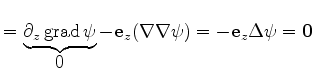
The first way for solving the partial differential equation system (5.18) and (5.19) is performed by a gradient field
| (5.24) |
| (5.25) |
 |
(5.29) |
 |
(5.30) |
Different to the previous way, the basic approach is a vector potential
| (5.31) |
The boundary conditions (5.26) and (5.27) result to
 |
 |
(5.37) |
| (5.38) |
 |
(5.39) |
 |
 |
The field lines of
![]() are defined by the differential equation
are defined by the differential equation
 |
(5.41) |
| (5.42) |
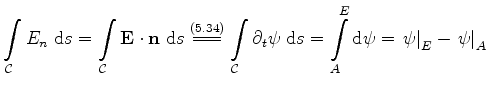
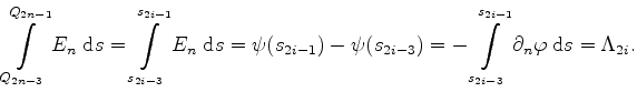
This derivation has shown that the duality of the field lines and equipotential lines within the given set of differential equations can be obtained by a replacement of Dirichlet (homogenous Neumann) by homogenous Neumann (Dirichlet) boundary conditions. The values of
![]() have to be evaluated by (5.28) and (5.43).
have to be evaluated by (5.28) and (5.43).
In this generalization of the capacitor problem, even more than two electrodes in the original constellation could be handled. In this case, if the original field problem has ![]() boundaries with imposed voltage, it requires also
boundaries with imposed voltage, it requires also ![]() Neumann boundaries (electrodes for the dual system) which alternate with the Dirichlet boundaries along the whole surface.
Neumann boundaries (electrodes for the dual system) which alternate with the Dirichlet boundaries along the whole surface.
As neither a bias of ![]() nor an arbitrary constant scaling factor of
nor an arbitrary constant scaling factor of ![]() change the shape of the field lines (equipotential lines of
change the shape of the field lines (equipotential lines of ![]() ), in case of exactly two contacts, the actual values of the two dual boundary voltages can be set to two different arbitrary values, most notably to values suitable for the computation.
), in case of exactly two contacts, the actual values of the two dual boundary voltages can be set to two different arbitrary values, most notably to values suitable for the computation.
Unfortunately such a duality is not guaranteed in three dimensions. The theoretical expansion of the two-dimensional capacitor model delivers a three-dimensional capacitor with six sides where two of them act as electrodes. To determine the field lines, three potentials have to be calculated: one with the original electrode setting, one with two other opposite electrodes and the third one with the remaining two opposite electrodes.
One might expect that the expanded two-dimensional duality formulation can be expressed as follows:
The three fields build an orthogonal system. The field lines of each electric field lie within the equipotential surfaces of each of the remaining potentials and the conclusion is that the intersections of two equipotential surfaces deliver the field lines of the third potential.Nevertheless, this might not hold under certain circumstances. In three dimensions, the duality formulation is not guaranteed, because the three potentials, which can be considered as a curvilinear coordinate system, usually do not represent an orthogonal system. Particularly, it is not even guaranteed that the field lines on the surface of the simulation domain are the equipotential lines of one of the other potentials. Additionally, the different electric fields are not perpendicular [70].
![\includegraphics[width=9cm]{picsconveps/surf11}](img569.png)
![\includegraphics[width=5.0cm]{picsconveps/coord2}](img570.png)
|
The orthogonality of the equipotential surfaces only exists, if the coordinate lines on the surface follow lines of curvature. This happens, when the coordinate lines follow surface lines of maximum or minimum curvature. However, this is only fulfilled for simple geometries and usually not satisfied [70].
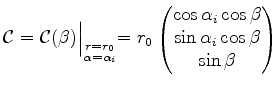
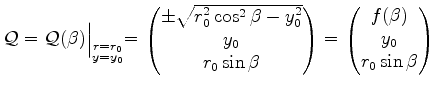
The following example should clarify the situation. Consider a spherical device region as shown in Figure 5.13. The coordinates of the device are given in spherical coordinates by
![$\displaystyle \begin{pmatrix}x\ y\ z\end{pmatrix}=r \begin{pmatrix}\cos \alpha \cos \beta\ \sin \alpha \cos \beta\ \sin \beta\end{pmatrix}. \pagebreak[4]$](img571.png) |
(5.43) |
Constant radius
![]() delivers the surface of this domain.
The meridians of the sphere are formed by
delivers the surface of this domain.
The meridians of the sphere are formed by
![]() and
and
![]() and represent circles of constant height.
The upper and lower contacts of the domain of the capacitor are cups of the sphere and will be limited by the circles at
and represent circles of constant height.
The upper and lower contacts of the domain of the capacitor are cups of the sphere and will be limited by the circles at
![]() and
and
![]() . The extracted potential is
. The extracted potential is ![]() .
With this contact setting the solution is rotationally symmetric and it follows that
the equipotential lines at the surface of the sphere are circles of constant height
.
With this contact setting the solution is rotationally symmetric and it follows that
the equipotential lines at the surface of the sphere are circles of constant height
![]() and the field lines at the surface are meridians between
and the field lines at the surface are meridians between ![]() and
and ![]() with
with
![]() .
.
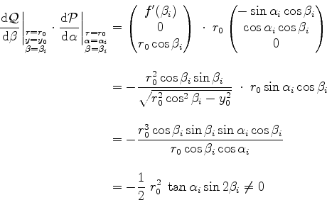
Inside the device, the equipotential surfaces are perpendicular to the surface of the sphere and the field lines are also perpendicular to the former. Fortunately, a complete analytical solution of the potential distribution is not necessary.
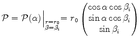
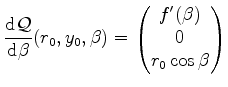
The major prediction is that the field lines at the surface of the sphere
![]() are represented by meridians
are represented by meridians
 |
(5.44) |
 |
(5.45) |
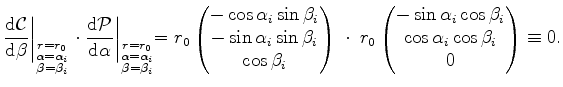 |
(5.46) |
So far, there was no specification of the other four electrodes. However, any possible specification of them does not change the layout of the original field lines.
The second potential ![]() is defined by the left and right electrodes as the cup of the remaining part of the sphere at
is defined by the left and right electrodes as the cup of the remaining part of the sphere at ![]() and
and ![]() . The front and back contacts are the remaining parts of the surface and deliver the potential
. The front and back contacts are the remaining parts of the surface and deliver the potential ![]() .
The borderline of the left contact and the front contact is a line of constant y-coordinate
.
The borderline of the left contact and the front contact is a line of constant y-coordinate
 |
(5.47) |
 |
(5.48) |
 |
(5.49) |
Nevertheless, usually even these surfaces will be nearly orthogonal, within the geometries considered and due to the smoothness of the resulting potential lines arising from the Laplace equation. Therefore, nearly cuboidal elements and smooth grids will be produced by the equipotential surfaces. The equipotential surfaces conform to the boundaries. As a result all points inside the simulation area will be reached by the equipotential surfaces of
![]() ,
,
![]() and
and
![]() -- a geometrical point
-- a geometrical point ![]() inside the simulation domain can be described by a triple
inside the simulation domain can be described by a triple
![]() . Only in rare cases, an ambiguous mapping, a folding of the curvilinear coordinate lines, may arise [36][70].
. Only in rare cases, an ambiguous mapping, a folding of the curvilinear coordinate lines, may arise [36][70].
|
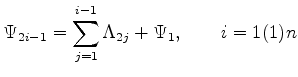
By selecting several potential value ticks of the three different potentials and calculating the intersection points of the equipotential surfaces, the point set for the grid generation is derived. With the selection of the tick values of the potentials, the grid density can be controlled in various ways.
To simplify the expressions, the boundary values of the potentials are set to 0 and ![]() .
Each geometrical point
.
Each geometrical point ![]() inside the capacitor has a potential representation
inside the capacitor has a potential representation
![]() within the potential range
within the potential range
![]() . As the discrete maximum principle is satisfied, it seems plausible that the potential values raise monotonously along the field lines, going from one electrode to the opposite one. Therefore, except for folding it is a one-one mapping of geometrical points to potential coordinates.
In this way, a selected potential triple
. As the discrete maximum principle is satisfied, it seems plausible that the potential values raise monotonously along the field lines, going from one electrode to the opposite one. Therefore, except for folding it is a one-one mapping of geometrical points to potential coordinates.
In this way, a selected potential triple
![]() delivers a distinct geometrical point
delivers a distinct geometrical point ![]() inside the capacitor.
inside the capacitor.
In a first step it is necessary to find an initial Delaunay tetrahedrization of the capacitor domain. This grid generation step does not need a special grid refinement. All material properties are linear, in particular a constant permittivity is used, and the Laplace equation as an elliptic partial differential equation is numerically well behaved. In addition, as a big advantage different from generating a grid for the whole device, only one capacitor segment has to be meshed. This grid can be produced regardless of other segments. This means that no additional grid points are induced by geometry and grid constrains of neighboring segments. A relatively crude grid can be used. Only for preserving the quality of the resulting cuboids, it is useful to introduce a refinement criterion based on the directions of the electric fields.
The solutions of the field equations is usually obtained by the Box Integration method (refer Section 3.1). The differential equation systems for solving the three potential distributions can be seen in Figure 5.1. The resulting equation system is of the form
| (5.50) |
| (5.51) |
The elements of the system matrix
![]() and the right-hand side
and the right-hand side
![]() are set to
are set to
 |
(5.52) |
 |
(5.53) |
| (5.54) |
| (5.55) | |
| (5.56) |
| (5.57) | |
| (5.58) |
These equations are used for calculating for the potential values ![]() on the grid points
on the grid points ![]() . For the potentials
. For the potentials ![]() and
and ![]() an similar equation system is set up. Basically, all three potential evaluations use the same system matrix
an similar equation system is set up. Basically, all three potential evaluations use the same system matrix
![]() , except the lines and rows resulting from the boundary points where the adequate boundary conditions have to be inserted.
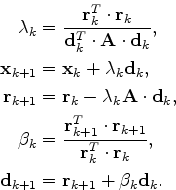
For the evaluation of the potential values, a Conjugate Gradient Solver is advisable [71].
, except the lines and rows resulting from the boundary points where the adequate boundary conditions have to be inserted.
For the evaluation of the potential values, a Conjugate Gradient Solver is advisable [71].
The matrix ![]() , for the equation system
, for the equation system
![]() , is a sparse
, is a sparse ![]() matrix.
Applying a Gaussian Solver destroys the sparse system, because by eliminating the entries under the diagonal a lot of entries above the diagonal become non-zero.
Therefore, the memory usage for storing the system matrix elements increases to
matrix.
Applying a Gaussian Solver destroys the sparse system, because by eliminating the entries under the diagonal a lot of entries above the diagonal become non-zero.
Therefore, the memory usage for storing the system matrix elements increases to
![]() .
Additionally the elimination of a fully occupied row requires
.
Additionally the elimination of a fully occupied row requires
![]() arithmetic operations and eliminating all rows is of
arithmetic operations and eliminating all rows is of
![]() .
Therefore the use of a solver, which preserves the sparsity of the system and does not show a complexity of
.
Therefore the use of a solver, which preserves the sparsity of the system and does not show a complexity of
![]() is a better choice.
With simple modifications, the system matrix
is a better choice.
With simple modifications, the system matrix
![]() can be made suitable for a Conjugate Gradient solver.
Since a CG-solver requires a symmetrical system matrix, the original matrix must be transformed to become symmetric. The symmetry of the system matrix is violated in rows and columns where the values of
can be made suitable for a Conjugate Gradient solver.
Since a CG-solver requires a symmetrical system matrix, the original matrix must be transformed to become symmetric. The symmetry of the system matrix is violated in rows and columns where the values of ![]() are imposed. One possible method is to pre-eliminate these rows and columns and move the adequate entries to the right-hand side. This method requires a row number to point number remapping and each potential system delivers a completely different system matrix.
are imposed. One possible method is to pre-eliminate these rows and columns and move the adequate entries to the right-hand side. This method requires a row number to point number remapping and each potential system delivers a completely different system matrix.
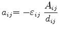
Another way is to eliminate asymmetrical matrix entries ![]() on the left-hand side by
on the left-hand side by
 |
(5.60) |
 |
(5.61) |
![]() with
with
![]() and
and ![]() on
on
![]() or on
or on
![]() .
.
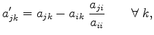
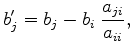
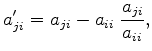
As all off-diagonal elements ![]() with
with ![]() of the concerned rows are zero, the transformation does not change any other entries than
of the concerned rows are zero, the transformation does not change any other entries than ![]() and simplifies to
and simplifies to
 |
(5.62) |
|
(5.63) |
![]() with
with ![]() and
and ![]() on
on
![]() or on
or on
![]() .
.
For an efficient memory representation of the equations, it is necessary to use a sparse matrix representation. The chosen method is only practicable, if the matrix values are left unchanged during the whole solving process and direct access to the row entries can be omitted. This representation can be assembled easily by iteration over all points and insertion of the couplings of the edges that are connected with the iteration point. The storage representation of a matrix works with four arrays diag[], offdiag[], colidx[], startcolidx[], where the entries are defined as [49]:
|
Algorithm
5.3.1 Sparse representation of
|
With this method, matrix-vector products can be performed directly on this data structure. Direct access to the row indices can be omitted by using the following algorithm:
No special sorting of the column indices is necessary. Matrix-matrix products, however, require direct access to the row entries within the above matrix representation and thus a search algorithm within the row indices becomes necessary. This kind of products has to be avoided. Therefore, a simple CG-algorithm without pivoting and without preconditioning is used. The algorithm looks as follows:
 |
In this case, only vector-vector products (
![]() ) and matrix-vector products are needed.
If only the non-zero entries of the matrix
) and matrix-vector products are needed.
If only the non-zero entries of the matrix ![]() are stored, the memory usage is of the same order as the number of existing edges
are stored, the memory usage is of the same order as the number of existing edges ![]() . The number of arithmetic operations for a matrix-vector product is of
. The number of arithmetic operations for a matrix-vector product is of
![]() , too.
With the use of exact arithmetic, the equation solver delivers the solution at least after
, too.
With the use of exact arithmetic, the equation solver delivers the solution at least after ![]() recursion steps. With non-exact arithmetic a border for the residuum
recursion steps. With non-exact arithmetic a border for the residuum
![]() must be given and usually this border is reached with less than
must be given and usually this border is reached with less than ![]() steps [20][63][71].
steps [20][63][71].
While the mean value of edges in a tetrahedral mesh is of the same order than the number of grid points (usually multiplied with a typical factor, but surely not of quadratic or higher order), the matrix-vector product is also of
![]() .
Therefore the memory usage is of
.
Therefore the memory usage is of
![]() and the amount of arithmetic operations for solving the equation system is of order
and the amount of arithmetic operations for solving the equation system is of order
![]() , which is a huge improvement compared to a Gaussian solver.
, which is a huge improvement compared to a Gaussian solver.
![\includegraphics[width=12cm]{picsconveps/isofield.eps}](img472.png)
![\includegraphics[width=12cm]{picsconveps/el22}](img479.png)
![\includegraphics[width=13cm]{picsconveps/p2}](img487.png)
![\includegraphics[width=13cm]{picsconveps/p0}](img488.png)
![\includegraphics[width=13cm]{picsconveps/p1}](img489.png)
![\includegraphics[width=14cm]{picsconveps/proof}](img516.png)
![$\textstyle \parbox{8.8cm}{\includegraphics[width=8.8cm]
{picsconveps/mehrere}}$](img596.png)
![$\textstyle \parbox{8.8cm}{\includegraphics[width=8.8cm]
{picsconveps/nureine}}$](img597.png)