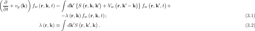
The WBE, introduced in Chapter 2, is written here as
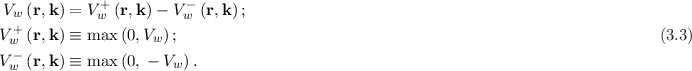
The Wigner potential can be decomposed as
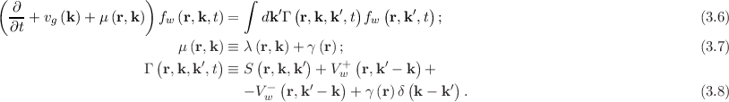
The quantity, which will emerge to be the scattering rate associated with the Wigner potential, is defined asThe term γ fw
fw is added to both sides of (3.1), such that

The partial differential equation represented in (3.6) can be transformed into an ordinary differential equation by introducing the characteristics of the Wigner function, which correspond to Newton trajectories in the physical sense. The trajectory of position (assuming parabolic bands and no electro-magnetic fields) can be parametrized with τ as
The trajectory Rn is initialized by the values  (which represent values in this context and not variables). Depending on the choice of the initialization time
tn, the trajectory is either forward in time
(which represent values in this context and not variables). Depending on the choice of the initialization time
tn, the trajectory is either forward in time  or backward in time
  . The trajectory of the wavevector is constant, since the LHS of (3.1) does not have
a force term that accelerates the particle and is formally introduced as
. The trajectory of the wavevector is constant, since the LHS of (3.1) does not have
a force term that accelerates the particle and is formally introduced as

The LHS of (3.6) can represent the full derivative of fw (with respect to parameter τ). To achieve this, the following property, for an arbitrary function g, is used:
such that

The value of b (integration limit) can be chosen freely and is chosen as t0 in the following.
Both sides of (3.6) are multiplied by the term exp to yield
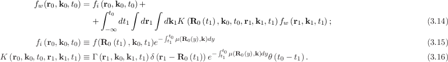
 to finally yield the integral form of (3.6):
This equation evaluates the Wigner function at the phase space point
to finally yield the integral form of (3.6):
This equation evaluates the Wigner function at the phase space point  at time t0 using the initial condition fw,i
 = fw(R
 ,k,t), which is
assumed to be known at time t.
,k,t), which is
assumed to be known at time t.
The integral equation (3.12) has a form analogous to the Chamber’s path integral [115], but with the contributions of the Wigner potential added. The introduction of the exponential term in (3.11) actually relates to an analytical summation of all out-scattering – the term μ could, alternatively, also be retained on the RHS of (3.1) and integrated otherwise, thereby suppressing the exponential term. However, the form of (3.12) is preferable as it gives a clear physical interpretation, which is useful when devising the Monte Carlo algorithm (Section 3.6).
The exponential term e-∫
tt0μ dy gives the probability of a particle to remain on its trajectory, i.e. not be scattered, from time t until time t0. Therefore, the
first term of (3.12) gives the contribution of particles initialized at
dy gives the probability of a particle to remain on its trajectory, i.e. not be scattered, from time t until time t0. Therefore, the
first term of (3.12) gives the contribution of particles initialized at  to reach point
  without being scattered, whereas the second term gives the
contribution of all particles scattered into the appropriate trajectory (according to in-scattering rate Γ) at time t′ to remain on the trajectory to reach point
without being scattered, whereas the second term gives the
contribution of all particles scattered into the appropriate trajectory (according to in-scattering rate Γ) at time t′ to remain on the trajectory to reach point  at
time to.
at
time to.
Fredholm integral equations of the second kind1 have the form:
where the free term fi and the kernel K are known and describe the initial/boundary conditions and the propagation of particles, respectively; Q is a multi-variable representing e.g. .
.
To express (3.12) in the form of (3.13), the integral must be augmented by the
variable2 r1
to complete Q1 =  :
:
A very wide variety of physical phenomena can be described by integral equations of the form (3.13) and a strong theory has evolved surrounding the solution of such Fredholm integral equations using Monte Carlo algorithms [117].
It is possible to formulate an integral representation of the WBE for the entire (global) domain. Sometimes, however, the operator of the equation under consideration is too complicated to be able to formulate a global integral representation. In such a case, local integral representations are used based on the Green’s function3 Monte Carlo algorithm [105]. The theory of Green’s function Monte Carlo algorithms keeps on developing [118, 119, 120] and is often applied to solve non-linear physical problems, e.g. [121].
The adjoint form of integral equations, of the form as in (3.13), is often easier to solve [106, 122].
The integral form of the WBE in (3.12) and (3.14) describes a backward-in-time equation as seen from the limits of the time integral. To obtain the corresponding forward-in-time equation the adjoint equation is required [123].
The kernel of (3.13) can be interpreted as a propagator: K describes the propagation from Q1 to Q. The adjoint equation to (3.13) solves for the function g
(to which no particular physical meaning is attached at this stage) and uses the (self-)adjoint kernel K†
describes the propagation from Q1 to Q. The adjoint equation to (3.13) solves for the function g
(to which no particular physical meaning is attached at this stage) and uses the (self-)adjoint kernel K† = K
= K , which exchanges the position of the
integration variable:
, which exchanges the position of the
integration variable:
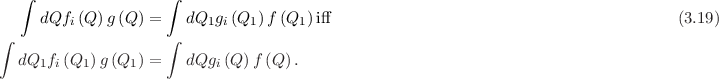
Using the newly introduced adjoint equation it can be shown that
This result is obtained, if (3.13) is multiplied by g(Q) and integrated by ∫ dQ and (3.17) is multiplied by f(Q1) and integrated by ∫ dQ1; the two resulting equations are subtracted. It follows