Overview of carrier transport models

1.2 Overview of carrier transport models

Semiconductor devices and nanostructures are open systems that interact with their environment, e.g. through leads/contacts, phonons or electromagnetic fields. The effect of these interactions, especially the electric field created by the voltage applied between the contacts¹ , is so strong that the statistical distribution of particles (charge carriers) strongly deviates from the statistics applicable in equilibrium, e.g. the Fermi-Dirac distribution. The results of linear response theory, e.g. the relaxation time approximation, are no longer sufficient for an accurate description [6, 7]. The non-equilibrium distribution can be determined by solving a transport equation which describes the movement of particles under the influence of external forces.

There exists a plethora of transport models, each having its limitations and advantages. The choice of a model depends on the application (phenomena) to be simulated and the computational resources/time available. From a physical point of view it is attractive to choose the most fundamental models, but these may not computationally feasible, nor required, for a given task. The aim of this section is to provide an overview of the most important transport models used for semiconductor devices and nanostructures. The capabilities and limitations of the models are highlighted to be able to appreciate the position and capabilities of transport simulations based on the Wigner formalism.

In the following the most important semi-classical transport models will be covered first, because they still find application today in nanoscale devices when augmented with quantum models/corrections. Thereafter, the full-fledged quantum transport models are introduced. The considerations are presented based on intuitive concepts, like particles and distribution functions, which characterize the historical evolution of the field of transport models. Many of these classical attributes are retained in the Wigner formalism which bridges the two limiting transport regimes (semi-classical/diffusive and quantum/coherent) presented hereafter.

In the following a single-particle description is deemed sufficient to describe a particle ensemble in a statistical manner [8]. Moreover, only interactions between different kinds of particles are considered, e.g. electron with phonons. Many-particle phenomena, like Coulomb interaction, that occur between particles of the same kind are not considered explicitly and are only accounted for via the Poisson equation.

1.2.1 Classification of transport models

The physics that governs carrier transport depends on three characteristic lengths as related to the dimensions of a device [9]:

De Broglie wavelength: the wavelength associated to a particle with a momentum p by λ =∕_h. For an electron in silicon at room temperature λ ≈ 8nm [8], whereas in GaAs λ ≈ 17nm [10].
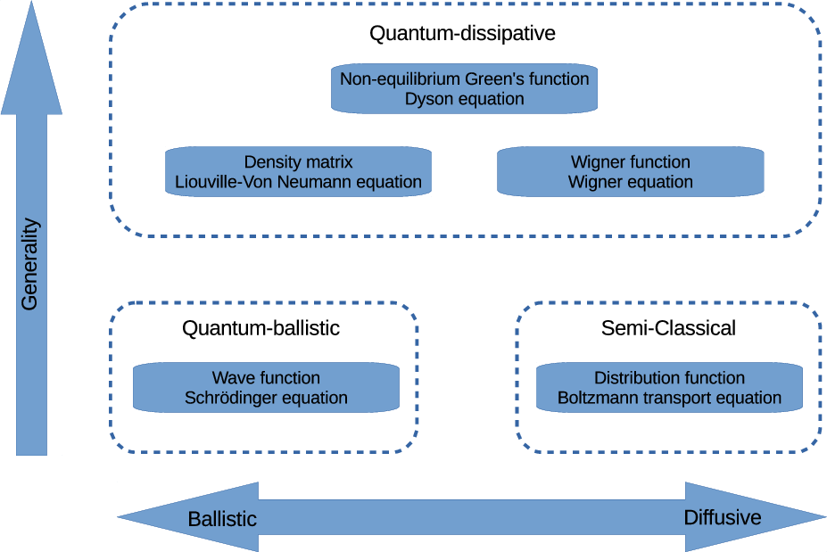
Mean free path (MFP): the mean distance a carrier travels before a momentum-altering scattering event occurs, e.g. inelastic phonon scattering. The MFP depends on the electric field but is in the order of 5-10nm for an electron in silicon at room temperature and up to an order of magnitude longer for GaAs [11, 12].
Phase relaxation length (PRL): the mean distance a carrier travels before a phase-changing scattering event occurs, e.g. electron-electron scattering. In semiconductors the relation between the PRL and the MFP depends on the type of semiconductor [13], but the PRL usually matches or exceeds the MFP [9].

Considering the above, one can distinguish between two limiting cases: the diffusive regime where the size of the device is much larger than all the characteristic lengths and carrier transport is predominantly determined by the scattering taking place; the other extreme, in devices shorter than all the characteristic lengths, is the ballistic regime where negligible scattering occurs and the transport is completely coherent² . Whereas transport in the diffusive regime can be appropriately described by semi-classical transport models, the ballistic regime requires models which consider the coherent wave nature of particles. The transition between the diffusive and the ballistic regime is gradual and nanostructures/devices, where both scattering and coherent transport play a role, demand the most general transport models, as is illustrated in Figure 1.1 (based on [14]).

An interplay between diffusive and coherent transport is often encountered in mesoscopic devices with at least one dimension shorter than one of the characteristic lengths mentioned above. In such devices quantum processes are at play that can be observed macroscopically, e.g. conductance fluctuations [15].

Quantization effects, due to confinement, start to appear, if at least one physical dimension of a device is below the De Broglie wavelength of the carriers. Interference effects imply coherent transport and become significant if the PRL exceeds at least one dimension of a device. Since the PRL can exceed the MFP in semiconductors, the phase coherence can be retained despite scattering taking place.

Figure 1.1: Overview of microscopic transport models. A distinction is made between models that can only describe only ballistic or diffusive transport and more general models which can describe transport in both regimes.

Apart from the physically-grounded distinction between transport models between the ballistic and diffusive regimes, the models can further be classified as either microscopic or macroscopic. Microscopic transport models describe the evolution of the distribution function (semi-classical) or state (quantum) of the system, from which all physical quantities (observables) of interest can be calculated. Macroscopic models are derived from the microscopic transport equations and directly solve for physical quantities – often termed engineering quantities – like electron concentration or current density. The computational efficiency afforded by macroscopic models comes at the cost of a loss in generality – certain assumptions are made, which limit the scope where the models remain valid. A thorough treatment of the mathematical derivations of both semi-classical and quantum macroscopic models is given in [8].

A hierarchy of models can be set up ranging from, at the most fundamental level, a quantum microscopic model to a semi-classical macroscopic description of carrier transport. Table 1.1 presents such a hierarchy, along with the device dimensions and applications at which each model is applicable.

Table 1.1: Hierarchy of carrier transport models incorporating dissipative interactions with typical active region of devices and the physical quantity which governs the device physics.

Model	Active region	Governed by
Non-Equilibrium Green’s Function	< 10nm	Potential
Density matrix / Wigner	< 100nm	Potential
Boltzmann	< 1μm	Sharp field
Hydrodynamic / Energy transport	100nm ÷ 1μm	Sharp field
Drift-diffusion	> 1μm	Smooth field

1.2.2 Poisson equation

The Poisson equation describes the electrostatics in a device based on the distribution of charges. A self-consistent solution³ of the Poisson equation with the transport models takes the long-range Coulomb interaction – a many-identical-particle effect – into account.

The Poisson equation follows from Gauss’s law, which relates the divergence of the electric displacement vector to charge density. The electric field displacement vector can be related to the electrostatic potential under the assumption of a time-independent permittivity, a negligible magnetic field and no polarization effects [16]. These assumptions are reasonable for many semiconductor devices for which the Poisson equation is defined as

∇ ⋅(- κ∇V ) = ρc, (1.1)

where κ, V and ρ_c denote the dielectric permittivity, electrostatic potential and charge density, respectively. The charge density is typically determined by free charge carriers and ionized impurities in the semiconductor.

In semiconductor materials with very strong polarization effects, e.g. galliumnitride, or devices where piezoelectric or ferromagnetic phenomena come into play, the Poisson equation, in the form of (1.1) is no longer sufficient [16].

1.2.3 Semi-classical models

The Boltzmann transport equation (BTE) has been the cornerstone of semi-classical device TCAD for many years and appropriately describes carrier transport in the diffusive regime. The BTE is introduced here and will be referred to again in Chapter 2, where accompanying scattering models are used to augment the Wigner transport equation.

The BTE is classified as semi-classical, because the treatment of carrier transport is classical (Newtonian), but some quantum concepts are considered, like the band structure (in the group velocity) and the Pauli exclusion principle (in the collision operator). The BTE provides microscopic insight into device operation but its high dimensionality makes its solution computationally expensive. Various macroscopic models, e.g. drift-diffusion, can be derived from the BTE and directly solve macroscopic quantities, thereby greatly reducing the numerical complexity of the simulation.

1.2.3.1 Boltzmann transport equation

The BTE describes the evolution of the distribution function f (r,k,t) , which gives the number of particles per unit volume of the phase space at time t. The phase space encompasses all possible values of the position r and the wavevector k (related to the crystal momentum by p = ℏk) that a particle can attain.

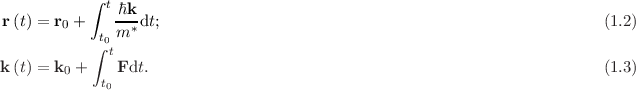
The movement of a particle in the phase space is described by its Newton trajectories, parametrized in time and initialized at the point (r0,k0) at t₀:

∫ t r(t) = r0 + ℏk-dt; (1.2) t0 m * ∫ t k (t) = k0 + Fdt. (1.3) t0

The (differentiable and conservative) force is defined as

dk-(t)- F = ℏ dt = - e(E + vg × B ), (1.4)

where e, E and B denote the magnitude of an elementary charge, electric field and magnetic field, respectively. The group velocity is given by

dr(t)- -1 vg = dt = ℏ ∇k ϵ(k), (1.5)

where ϵ

denotes the dispersion relation.

The Liouville theorem states that along the Newton trajectories the distribution function remains constant, i.e.

df = ∂f-+ dr(t)∇ f + dk-(t)∇ f = 0. (1.6) dt ∂t dt r dt k

This is known as the Vlasov equation [8] and describes the evolution of the distribution function. The spatial gradient term ∇_rf accounts for driving forces due to diffusion, thermoelectric and thermomagnetic effects. All external forces are encompassed in the term dk(t)
dt

The Vlasov equation gives an exact description of a semi-classical carrier moving in a perfect lattice; all lattice-carrier interactions are accounted for through the group velocity v_g, which depends on the band structure of the semiconductor lattice through the dispersion relation ϵ (k) . Lattice imperfections, lattice vibrations (phonons) and carrier-carrier interactions, however, introduce internal forces in the lattice which perturb the motion of the carriers. These perturbations in the trajectory of a carrier are known as collisions and are described by statistical laws (in the form of a collision operator), because an explicit consideration by the laws of dynamics is not feasible [16].

The collision operator augments the right-hand side of (1.6) and describes the effect of collisions on the distribution function such that

df = Cˆ[f (r,k,t)]. (1.7) dt

The collision operator Ĉ [⋅] is given by

∫ { ( ) ( ) ( )} Cˆ[f (r,k,t)] = f k′ S k ′,k - f (k )S k, k′ dk′ (1.8)

and describes the scattering rate of carriers into (from) a state with wavevector k (k′) from (into) a state with a wavevector k′ (k). The Pauli exclusion principle (not included here) prescribes that the in- and out-scattering only takes place if the final states are available. However, this is a many-identical-particle effect [7] and consequently is omitted in (1.8). The neglect of the exclusion principle is reasonable under non-degenerate conditions (low carrier density).

The scattering rate between the states of different wavevectors is specified by the function S, which compounds the expressions describing the various scattering mechanisms, e.g. carrier-phonon interactions, which change the momentum of a particle and make the system dissipative. The scattering rate for a specific mechanism is calculated using overlap integrals [7]. A more detailed treatment of the scattering models is given in Chapter 2.

The consideration of collisions, through the collision operator (1.8), in the Vlasov equation (1.6) yields what is known as the Boltzmann transport equation:

{∂f + v ∇ f + F∇ f = ∫ {f (k′,t)S (k ′,k) - f (k,t)S (k,k′)}dk′ ∂t g r k (1.9) f (r,k,t0) = f (r0,k0)

An initial condition at t₀ must be specified to have a well-posed problem.

The mean value ⟨AT⟩ of any physical quantity A (r,k) , like carrier concentration or energy, at time t = T can be calculated, if the distribution function is known:

∫ ∫ ⟨AT ⟩ = drdkA (r,k)f (r,k,T ). (1.10)

For instance, the carrier concentration for a volume Ω can be calculated by

∫ n (r) =-1 dkf (r,k) (1.11) Ω

and the current density as

∫ J (r) = - e dkf (r,k) vg(k). (1.12) Ω

The validity of the BTE rests upon the assumptions [17] that

point-like particles are exactly localized in the phase space and their transport is accurately described by the semi-classical Newton laws;
particle scattering takes place instantaneously at a fixed position, i.e. particles do not move during a scattering process.

From a quantum mechanical point of view the BTE fails to account for the quantum effects that appear due to the wave nature of charge carrier motion, like non-locality, interference and correlation effects. The fact that the momentum and position are defined exactly at the same time with f (r,k,t) makes the classical nature of the BTE obvious.

The Heisenberg uncertainty principle imposes limits on the range of validity of the BTE but they are not (yet) reached for most devices. The uncertainty relation ΔrΔp ≥^ℏ∕₂ requires that the potential within a device should change only negligibly over the De Broglie wavelength of the carriers. The latter, assuming an electron in silicon at room temperature, is in the order of 8nm [8]. Once the dimensions of the active regions of a device approach the De Broglie wavelength of the charge carriers, the BTE should be substituted by a wave equation to describe carrier transport [17].

A further constraint is given by the relation, ΔEΔt ≥ ℏ, which requires that the momentum relaxation time should be much smaller compared to the period of the operating frequency – this limits the validity of BTE to operation frequencies under approximately 6THz [17].

1.2.3.2 Macroscopic models

Macroscopic transport models can be formally derived from the BTE and have been extensively treated in the literature [17, 18, 19, 20]. The basic principle is to calculate moments of the BTE, which yields equations describing the conservation and flux of physical quantities, like mass, momentum or energy. A hierarchy of macroscopic models can be derived by considering moments of increasing order (in k), ranging from the drift-diffusion model to the six-moment model. In each case a so-called closure relation encapsulates the assumptions made on higher-order moments of the distribution needed to make the system of equations fully determined.

Drift-diffusion: The drift-diffusion (DD) model was originally proposed based on phenomenological arguments [21]. The derivation considers the first two moments of the BTE and assumes a cold Maxwellian for the distribution function as a closure relation. The resulting equations describe the conservation of mass – the carrier concentration n – and the flux of mass – the current density J_n:

1 ∂tn- -∇Jn = Gn; (1.13) e Jn = e(Dn ∇n - μnn ∇V ), (1.14)

where D_n and μ_n denote the material-dependent diffusion coefficient and carrier mobility, respectively. The net generation-recombination rate G_n relates to the scattering operator in the BTE. The solution of (1.13) and (1.14) directly yields the quantities calculated with the distribution function in (1.11) and (1.12).

The fast, robust numerical solvers available for the DD model in commercial and open source TCAD software makes it the (highly parametrized) workhorse of industry for daily engineering tasks. The self-consistent solution obtained with the Poisson equation is also routinely used as an initial guess to improve the convergence of more complex transport models. The DD model is suitable to simulate devices for which the mobility can be satisfactorily modelled as a function of the electric field and thermal effects (carrier heating) are unimportant. These conditions are often met in low-power devices with an active region exceeding 1μm.

Energy transport (hydrodynamic): The energy transport (ET) model⁴ was originally proposed in [22] to account for hot carrier effects, like impact ionization and velocity overshoot, occurring in devices smaller than 1μm. The ET model considers two additional moments of the BTE, compared to the DD model, and was formally derived in [23]. A multitude of derivations and closure relations for the ET model exist [8, 22, 24]. Compared to (1.14), the gradient of the carrier temperature enters the mass flux equation as an additional driving force of the current. The additional moments introduce equations which enforce the conservation of energy and define the energy flux.

Six moments: The six-moment model considers a further two moments of the BTE [18, 19]. The conservation of a third quantity, related to the kurtosis (skewness) of the distribution function, is enforced, which allows to better model hot carrier phenomena. However, the strong coupling between the equations and the choice of appropriate closure relations has made the realization of a robust numerical solver very challenging [25]. As a result the six-moment model has not found wide-spread use and remains largely of academic interest.

1.2.4 Quantum models

The passage to quantum mechanics is opened by abandoning the idea that the state of a particle is represented by a single point in the phase space (as done in the BTE). The Heisenberg uncertainty principle does not allow the exact specification of two conjugate quantities, like position and momentum, simultaneously. The minimum uncertainty is given by

ℏ- Δr Δp ≥ 2, (1.15)

where Δr and Δp refer to the uncertainty (or standard deviation) in position and momentum in a specific direction and ℏ is the reduced Planck constant.

There exists a plethora of quantum transport models. Certain formalisms may be better suited, or simpler, than others for a specific application and every formalism has its (dis)advantages from a computational point of view. The focus here shall be placed on the formulations which enjoy the most widespread use, namely the Schrödinger equation, density matrix and non-equilibrium Green’s function (NEGF). The essential aspects of each model are highlighted in the following to enable a comparison with the Wigner formulation which will be detailed in Chapter 2.

1.2.4.1 Preliminaries

Quantum mechanics relies on two important concepts to model physical systems: i) the state of the system is described by a vector in a complex Hilbert space and ii) observables which describe physical quantities, like energy, are represented by Hermitian operators which act on the state.

Vectors and Operators: The state vector can be expressed using an orthonormal basis formed by the eigenstates of the Hermitian operator (observable) under consideration:

∑ |ψ ⟩ = cj |ϕj ⟩,cj = ⟨ϕj| ψ ⟩, (1.16) j

where c_j is the projection of the state vector |ψ ⟩

on the basis vector |ϕ ⟩
j

. The basis vectors are obtained by solving the eigenvalue problem for the observable represented by the operator Â:

Aˆ|ϕj⟩ = aj |ϕj⟩. (1.17)

One can distinguish between pure states and mixed states. A pure state implies complete knowledge of the state a system is in; the classical equivalent would be to have a complete knowledge of the position and momentum of every particle in a system (i.e. no single-particle description). A mixed state, however, introduces some uncertainty and assigns a probability p_k to each possible pure state | ⟩
|ψk , where ∑ _kp_k = 1. This is the quantum equivalent of a distribution function.

A mixed state is to be distinguished from a mixture (superposition/linear combination) of states. While the former conveys the probability of a system being in a certain state, the latter describes a single state composed of two (or more) other states – an entangled state. In general one has incomplete information about the quantum system under observation and the initial state from which the evolution starts. However, the probability of a state occurring is often known from statistical distributions, e.g the statistical mixture of eigenstates of energy in thermal equilibrium. A mixed state allows to model this uncertainty. It should be noted that the uncertainty about the state of a system acts in addition to the uncertainty introduced by Heisenberg’s principle.

Picture and Representations: The so-called picture adopted in quantum mechanics refers to the state vectors and observables (linear operators) chosen to represent the physical state and dynamical variables of a system. The Schrödinger picture makes the state time-dependent with the evolution of the system whereas the observables remain unchanged; the Heisenberg picture is the converse⁵ . In the interaction picture the time evolution is split between the observable and the state [6] – this is useful if the Hamiltonian (observable) has a time-dependent part, e.g. phonon interactions.

The choice of the basis vectors used to represent the vectors and operators corresponding to the chosen picture is known as the representation. The value of a physical observable is independent of the representation chosen. The coordinate representation is usually the most intuitive due to the complex shape of the potential profile V (r) . The state vector projected in the chosen representation is known as a wave function.

Hamiltonian: A quantum system is described by a Hamiltonian which states the energy of a system, i.e. an observable. The Hamiltonian can encapsulate all interactions in the system under observation and interactions with external systems. The complexity of the Hamiltonian can be extended as needed to model the physics of interest or as computationally feasible. If adopting the interaction picture, the Hamiltonian can be separated in a part describing time-independent effects, e.g. the band structure, and a part describing the time-dependent perturbations to the Hamiltonian from the ’outside world’, e.g. interactions with time-varying electromagnetic fields:

ˆ ˆ ˆ H = H0 + Hint, (1.18)

where Ĥ₀ is the non-interacting part, which is assumed to be exactly solvable and Ĥ_int contains all the interactions, such as carrier-carrier, carrier-phonon, impurity scattering and so forth.

In a coordinate representation under the assumption of a parabolic dispersion relation with effective mass m^*, the Hamiltonian is expressed as

ˆH = - -ℏ2-∇2 + V (r) (1.19) 0 2m * r

and will be used throughout this text, unless specified otherwise. The potential V (r)

encapsulates the electrostatic potential (from mobile electrons, ionized impurities and externally applied voltages) and changes in the conduction band (e.g. at heterojunctions) and can be obtained from (1.1) as in the semi-classical case.

1.2.4.2 Schrödinger equation

The Schrödinger equation is the fundamental equation of motion describing the evolution of a pure quantum state |ψ⟩ in a system described by the Hamiltonian operator Ĥ:

iℏ-∂ |ψ⟩ = ˆH |ψ ⟩. (1.20) ∂t

The presence of an imaginary term alludes to the wave nature of the equation. The time-independent version of (1.20),

ˆ H |ψ⟩ = λ|ψ⟩ , (1.21)

presents a specific case of (1.17), which yields the stationary states |ψj ⟩

and associated eigenvalues λ_j (energies) of the Hamiltonian. A pure state does not necessarily correspond to an eigenvector of the observable. The state vector can expressed in terms of the resulting basis

∑ |ψ ⟩ = cj |ψj⟩ ,cj ∈ C. (1.22) j

Since a mixed state cannot be represented by a single vector, (1.20) must be solved for each possible state separately. Equation (1.20) can be expressed in a coordinate representation as

∂- iℏ ∂tψ (r,t) = Hψ (r,t). (1.23)

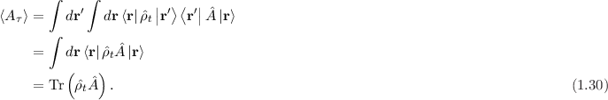
If the state is not an eigenstate of the observable, there is an uncertainty in the value which will be measured for the observable. The average of a physical quantity represented by an operator Â at time τ can be calculated by

∫ ˆ ˆ ⟨Aτ⟩ = ⟨ψ|A |ψ ⟩ = dr⟨ψt| r⟩⟨r|A |ψt⟩. (1.24)

Macroscopic quantities, like the probability density and current density, can be obtained from the wave functions forming the mixed state:

∑ n(r,t) = λj |ψj (r,t)|2; (1.25) j eℏ ∑ [ ] J(r,t) = - m-* λjIm ¯ψj (r,t)∇ ψj (r,t) . (1.26) j

The Schrödinger equation as presented above is applicable to a closed (bounded) system. To be useful for semiconductor devices the system must be ’opened up’ to allow the specification of boundary conditions, which gives rise to current-carrying (scattering) states. The quantum transmitting boundary method (QTBM) [26] allows the specification of the incoming flux from a lead to a device by a boundary condition for the wave function at the device/lead interface. The QTBM can provide the solution (wave function) inside the device and the transmission and reflection coefficients at the leads. Under the assumption of a constant potential in the leads, the form of solution in the leads is known to consist of incoming and outgoing waves and exponentially decaying evanescent waves along the interface. The QTBM employs this fact to specify boundary conditions at the lead/device interface expressed in terms of this known solution.

The Schrödinger equation is only well-suited to describe ballistic transport. Models for out-scattering, inspired by the relaxation time approximation, have been theoretically proposed (by adding an imaginary potential to the Hamiltonian), but numerical implementations have proven problematic [25].

1.2.4.3 Density matrix

The density matrix provides a convenient description of mixed states by specifying the relation between the states which comprise the mixed state.

The density matrix can be derived from the Schrödinger picture following the derivation in [20]. By adding unitary operators, expressed in the coordinate basis and the observable’s basis, (1.24) can be rewritten as

∫ ∫ ′ ( ′) *( ′) ⟨A τ⟩ = dr drα r,r ψ t r ψt(r). (1.27)

This introduces the density matrix

( ′ ) *( ′) ′⟩ ρ r,r,t = ψt r ψt(r) = ⟨r |ψt⟩⟨ψt| r (1.28)

with the corresponding density operator

ˆρt ≡ |ψt⟩ ⟨ψt|, (1.29)

which can be shown to be unitary using (1.22).

It follows that (1.27) can be expressed as

∫ ∫ | ⟩⟨ | ⟨Aτ⟩ = dr′ dr⟨r| ˆρt|r′ r′| ˆA |r⟩ ∫ = dr ⟨r| ˆρtAˆ|r⟩ ( ) = Tr ρˆAˆ . (1.30) t

Therefore, the expected value of a physical observable A can be calculated by applying the trace operator, which sums the diagonal terms of the resulting matrix.

Accordingly, the probability density can be calculated by

n(r,t) = 2Tr (ρt) = ρ(r,r,t) (1.31)

and the current density by

J(r,t) = iℏe lim (∇r′ - ∇r )ρ (r,r′,t). (1.32) m* r′→r

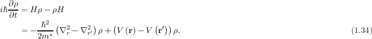
The Liouville-Von Neumann equation describes the evolution of the density matrix

∂ρ iℏ---= [H, ρ], (1.33) ∂t

where

denotes the commutator bracket and H the Hamiltonian defined in (1.19), such that

iℏ∂-ρ= H ρ- ρH ∂t ℏ2--( 2 2) ( ( ′)) = - 2m* ∇ r - ∇ r′ρ + V (r)- V r ρ. (1.34)

The density operator has a complete orthonormal set of eigenfunctions and eigenvalues, where each eigenpair can be associated with the solution of a Schrödinger equation. Therefore, a set of Schrödinger equations can also be used to represent a mixed state.

The introduction of a scattering operator in (1.34) which maintains the positive-definite character (physical validity) of the density matrix under all circumstances has proven challenging. Recently, the derivation of a more robust operator has been proposed [27], which has analogies with the scattering models for the Wigner equation (Chapter 2). However, due to the non-local nature of the density matrix, the models are more difficult to interpret.

1.2.4.4 Wigner function

For completeness the Wigner function is briefly introduced here. A thorough discussion is deferred to Chapter 2.

The Wigner function is obtained by applying the Wigner transform to the density matrix:

1 ∫ ′ ( r′) ( r′) fw (r,k, t) = ----3 dr′e-ik⋅rψ r- -- ψ* r + -- . (1.35) (2π) 2 2

Similarly, a Fourier transform of the Von Neumann equation for the density matrix (1.34) yields the evolution equation for the associated Wigner function:

∫ ( ) ( ) ∂-fw (r,k,t)+ -ℏk--∂-fw (r,k,t) = dk ′Vw r,k′ - k,t fw r,k′,t , (1.36) ∂t 2m *∂r

where V _w denotes the Wigner potential.

The Wigner function uses the phase-space variables, instead of the two spatial variables in the density matrix, which allows the scattering models from the Boltzmann transport equation to be adopted (to be discussed in Chapter 2).

1.2.4.5 Non-equilibrium Green’s function

The non-equilibrium Green’s function provides a general framework to describe weakly interacting quantum systems. It introduces a correlation in time in addition to the space correlation considered in the density matrix / Wigner function. Consider (1.28) for the case for which t≠t′: ρ (r,r′,t,t′) = ψ (r,t) ψ^* (r′,t′) . The Green’s function (assuming a coordinate representation) describes how the amplitude of a wave function (an excitation) at point r′ at time t′ is propagated to a point r at time t.

The time evolution of a wave function – the solution to the Schrödinger equation in (1.23) – can be calculated by

∫ ( ′ ′) ( ′ ′) ψ (r,t) = iℏ drG r,t,r,t ψ r,t . (1.37)

The Green’s function – also known as the propagator – can be viewed as a generalization of the scattering matrix, commonly used in radio frequency (RF) electronics, which relates the input and output at different ports, because it relates the response at an arbitrary point in the the system (device) to the excitation(s) at any other point(s).

The evolution of the time-resolved Green’s function is described by the Dyson equation [28], but its high dimensionality of 2d + 2 makes it numerically extremely challenging to solve in two and three spatial dimensions (d). Only very recently have such efforts even started [29, 30]. Therefore, the steady-state, where only the difference between the time variables appears, is considered in the following (as is routinely done in NEGF simulations).

A Fourier transform of the time difference t - t′ yields the energy E, which appears as parameter in the Green’s function G ′
(r,r;E ) ⁶ .

The Green’s function is calculated by solving the differential equation

[E - H (r)]G (r,r′) = δ(r - r′) , (1.38)

which permits two solutions, since the inverse of a differential operator, i.e. the Hamiltonian, is not uniquely specified without boundary conditions [9]. The two solutions correspond to a propagation forward and backward in time and are known as the advanced and retarded Green’s function, respectively. A unique solution arises once the boundary conditions are introduced in the form of a self-energy representing the effect of semi-infinite leads coupled to the device. In the following, the retarded Green’s function is implied without introducing additional notation.

The self-energy encompasses all possible interactions between the electron and its environment. Each interaction has its own self-energy, which is calculated using many-body perturbation theory under the presumption that systems are weakly interacting [28]. The self-energy accounting for the coupling of the device to semi-infinite leads reduces the system to a finite size and follows from similar arguments as used in the QTBM, i.e. plane waves are injected from a lead assumed to be at a constant potential. The calculation of the self-energies for other interactions, like phonon scattering, can become very computationally demanding and various approximations are routinely made to keep simulations tractable..

The coordinates in equation in (1.38) can be discretized and a representation in terms of matrices follows:

- 1 G = [EI - H - Σ ] , (1.39)

where I is the identity matrix, E denotes the energy, H is the Hamiltonian matrix and Σ is the self-energy matrix. The numerical task at hand is to invert the matrix in (1.39) for every energy value in the chosen range⁷ . Therefore, the size of the matrix should be kept as small as possible, which limits the size of devices which can be practically investigated.

The correlation function⁸ Gⁿ (r,r′,t,t′) is used to calculate physical observables and is related to the Green’s function G by

n in † G = GΣ G , (1.40)

where G^† is the Hermitian conjugate of G and Σⁱⁿ is the self-energy which accounts for in-scattering of electrons from leads and other interactions, like phonons. The function Gⁿ can be regarded as the quantum mechanical equivalent of the distribution function f in the semi-classical BTE.

Following [9], the electron and current density at a certain energy can be calculated by

n n (r,E) = G--(r,E-); (1.41) 2π J (r,E) = -ieℏ--1- lim (∇r - ∇r ′)Gn (r,E ). (1.42) 2m *2π r′→r

The total densities are obtained by integrating the expression (1.41) and (1.42) over all considered energy values and accounting for spin-degeneracy (multiplication by two).

The NEGF formalism is the most general of all the transport models reviewed here and is arguably the most popular formalism currently in use in the computational electronics community. However, the theoretical generality is accompanied by great computational demands and simplifications – as alluded to above – are routinely employed to make simulations numerically feasible. Therefore, the theoretical capabilities of a formalism should not be considered in isolation, but the extent to which these can be realized in simulations is equally important.

1.2.4.6 Quantum-corrected models

Quantum-corrected models refer to semi-classical models that are modified to capture important quantum effects. This allows the (relatively) computationally efficient semi-classical transport models to be used to approach the results obtained with a full-fledged quantum simulation. The modifications, however, introduce some fitting parameters which must be appropriately calibrated to a specific device to realise the desired improvements in accuracy.

The most prominent quantum effect in transistors is the quantization of energy levels. Spatial confinement leads to the separation of sub bands and is accompanied by an increase in interurban scattering, which can be accounted for by using degenerate statistics in Monte Carlo simulations of the BTE [31]. To calculate the true occupation of the discrete sub bands requires a self-consistent solution of the Schrödinger-Poisson system, but the charge distribution can be replicated in a semi-classical model using various approaches: The density of states (DOS) can be modified using various means, e.g. introducing a spatial dependence, or artificially modifying the energy band gap [31, 32].

A further option to account for the confinement effects is to apply a quantum correction to the potential [33]. There exists a multitude of models and derivations for the quantum potential [31, 34, 35], although all of them have a similar qualitative effect. The self-consistent potential obtained from semi-classical simulation is smoothed by a convolution with a Gaussian kernel. This effective potential indirectly models the uncertainty in the position of the electrons dictated by quantum mechanics using classical calculations and, therefore, can be applied to both the BTE and macroscopic models.

Quantum versions of the macroscopic models can also be derived from the Wigner(-Boltzmann) equation using the method of moments as done in the semi-classical case with the BTE. The corrective term (Ohm potential), as defined in [31], is simply added to the classical potential in (1.14) such that

( ( √ --)) -ℏ2- ∇2--n- Jn = e Dn ∇n - μnn∇ V - 2m * √n-- . (1.43)

The conservation equation for mass (1.13) is retained in the quantum DD model, but the additional gradient operators in (1.43) – hence, the name density gradient method – increase the order of the resulting partial differential equation and, therefore, additional boundary conditions must be specified. The use of a generalized electron quasi-Fermi potential can, however, reduce the order of the differential equation [36], which is preferable for a solution by numerical methods.

The density-gradient method has also been used to account for tunnelling effects in the gate stack and from source to drain [37]. The tunnelling effect can also be replicated in semi-classical models by introducing an additional generation (recombination) rate in (1.14) [38].

In addition to the expected computational efficiency, a further advantage of using quantum macroscopic models is that physically relevant boundary conditions are easier to specify than for the Schrödinger equation. The quantum-corrected models have been successfully applied for device simulation [35, 39], but some numerical challenges are faced with high-frequency oscillations which occur due to the dispersive nature of the equation [40].

Many approaches have been used to model quantum effects in a computationally efficient way by combining and modifying different equations, as sketched above. However, this ad hoc approach works well only for specific cases and lacks the generality of a full-fledged quantum model.

1.2.5 Summary

Whereas the relation between the semi-classical transport models is rather obvious – they all stem from the BTE – the relation between the different quantum transport models is slightly obscured by the use of different terms and terminology. Before the motivation for using Wigner-based transport models is given, it is valuable to briefly summarize and evaluate the models discussed up to now.

The semi-classical transport is based on the BTE and allows an accurate description in devices where transport takes place in the diffusive regime. Macroscopic models that directly solve for physical quantities can be derived from the BTE and are much less computationally demanding. Certain quantum mechanical effects can selectively be accounted for in semi-classical models with quantum-correction terms, but the quantum physics is not treated on a fundamental level.

A fundamental description of the wave nature of particles is required to describe quantum mechanical effects. The Schrödinger equation describes the evolution of a pure state and can describe the stationary states, but the inclusion of scattering is problematic. A generalization towards mixed states requires the density matrix, which describes the correlation between different states. The inclusion of scattering in the Von Neumann equation is possible, but the non-local nature makes the interpretation not very intuitive. The Wigner function is related to the density matrix through the unitary Fourier transform and gives a phase space description of quantum mechanics, which allows the adoption of familiar semi-classical scattering models. The most general formalism is the NEGF, which also takes time correlations into account. The high dimensionality of the Green’s function imposes significant computational demands, which makes the inclusion of scattering only tractable with simplifying assumptions.

[next] [prev] [prev-tail] [front] [up]