


Next: 2.2.2 Feature-Scale Transport
Up: 2.2 Transport Kinetics
Previous: 2.2 Transport Kinetics
Although process simulation in the reactor-scale region is not the scope of this work, some basic considerations of different transport models and typical characteristics of flux distribution on
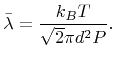
 are given in this section. The transport of particles can be characterized by the mean free path
 . For an ideal gas
calculates as [22]
. For an ideal gas
calculates as [22]
 |
(2.4) |
Here
 denotes the Boltzmann constant,
  is the temperature,
  is the pressure, and
  is the collision diameter of a gas molecule, which is about
 for most molecules of interest [91].
If the mean free path is much smaller than the representative physical length scale, which is true in the case of the reactor dimension, the transport is said to be in the continuum regime [32,80]. This is usually the case for CVD and dry etching processes with typical pressures in the range
 and a typical temperature of
 resulting in a mean free path in the range
 to
to
 . Hence, the velocities of a neutral particle species
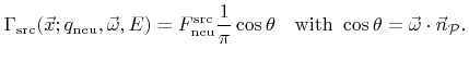
 can be assumed to follow the Maxwell-Boltzmann distribution, leading to a cosine-like directional dependence of the flux distribution on
 |
(2.5) |
Here the energy distribution is neglected, because the kinetic energy for typical process temperatures is usually too small to play a role in the surface reaction.  is the angle between the incident direction
 and
and
 .
.
 is the flux on
and can be assumed constant for all
is the flux on
and can be assumed constant for all
 at feature-scale. The value for
can either be obtained by calculating the reactor-scale transport or experimentally by measurements.
at feature-scale. The value for
can either be obtained by calculating the reactor-scale transport or experimentally by measurements.
In many processes plasmas are used, leading to the need to model ion transport. Ions are accelerated towards the wafer surface due to the plasma sheath potential. This leads to a narrow angle distribution often described as power cosine distribution [91], also known as Phong distribution in the field of computer graphics [90]
 |
(2.6) |
For large exponents  this is equivalent to a normal distribution
 with with |
(2.7) |
Together with the energy distribution
 where
where
 the arrival flux distribution can be expressed as
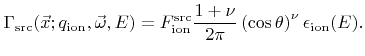 |
(2.8) |
If no collisions occur in the sheath, and if the final energy of ions is much larger than the initial random thermal energy,
 , the cosine exponent
can be estimated by [34]
, the cosine exponent
can be estimated by [34]
 |
(2.9) |
For direct current (DC) biased plasmas the final ion energy can be assumed to be monoenergetic with
 , where
 denotes the elementary charge and
 is the sheath potential. Hence, the energy distribution can be approximated by a Dirac delta function
 |
(2.10) |
Radio frequency (RF) biased plasmas result in more complex energy distributions with a characteristic bimodal shape. Plasma sheath simulations using MC techniques are able to predict the energy distribution function and can also incorporate ion collisions in the plasma sheath region [27,56].
For most processes the flux distribution
 does not vary significantly over
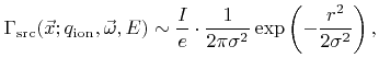
at feature-scale. However, this is not true for processes working with local particle bombardments such as FIBs. The spatial intensity distribution of such a beam is usually described by a Gaussian profile [57,132,133]
does not vary significantly over
at feature-scale. However, this is not true for processes working with local particle bombardments such as FIBs. The spatial intensity distribution of such a beam is usually described by a Gaussian profile [57,132,133]
 |
(2.11) |
where  denotes the beam current with typical values in the range
 to
to
 [99] and
  is the distance from the center line of the beam.
  is proportional to the beam diameter
, which is commonly defined as the full width at half maximum (FWHM), thus
is proportional to the beam diameter
, which is commonly defined as the full width at half maximum (FWHM), thus
 .
.
At feature-scale it is a reasonable approximation to regard the beam as monoenergetic and unidirectional. If  is the ion beam energy, typically ranging from
 [99], and if
 represents the incidence direction, the arrival angular energy flux distribution can be written as
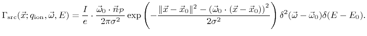 |
(2.12) |
Here  denotes a two-dimensional delta distribution satisfying
 .
.
Next: 2.2.2 Feature-Scale Transport
Up: 2.2 Transport Kinetics
Previous: 2.2 Transport Kinetics
Otmar Ertl: Numerical Methods for Topography Simulation