Instead of using an adaptive grid to represent the entire simulation domain, it is better to use a regular grid with an appropriate resolution and store only the LS values of defined grid points needed for the time integration scheme.
Run-length encoding along a certain grid direction is an efficient technique for this purpose [45]. In the following, run-length encoding is explained for the ![]() -direction. However, it can be applied to all other grid directions analogously. Each line of grid points parallel to the
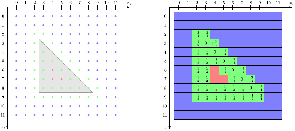
-direction. However, it can be applied to all other grid directions analogously. Each line of grid points parallel to the ![]() -direction is separately run-length encoded. Consecutive undefined grid points, for which the LS values do not need to be stored, are combined in runs. It is advantageous to use two different run codes, depending on whether the corresponding run contains only grid points where the LS function is positive or negative, respectively. In this way the sign of the LS function is available for all grid points. This information is useful, since it reveals on which side of the surface a grid point is located.
-direction is separately run-length encoded. Consecutive undefined grid points, for which the LS values do not need to be stored, are combined in runs. It is advantageous to use two different run codes, depending on whether the corresponding run contains only grid points where the LS function is positive or negative, respectively. In this way the sign of the LS function is available for all grid points. This information is useful, since it reveals on which side of the surface a grid point is located.
To demonstrate, run-length encoding is applied to the two-dimensional example shown in Figure 3.3. There, a triangle is described by the LS. The LS function is resolved on a grid with extensions
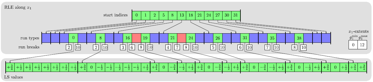
![]() . Figure 3.4 shows the corresponding run-length encoded (RLE) data structure which consists of 4 arrays in order to store only the LS values of defined grid points near the boundary. To address array entries, zero based indexing is used.
. Figure 3.4 shows the corresponding run-length encoded (RLE) data structure which consists of 4 arrays in order to store only the LS values of defined grid points near the boundary. To address array entries, zero based indexing is used.
|
|
The LS values of all defined grid points are stored in lexicographical order in the LS values array. Sequences of positive undefined, negative undefined, or defined grid points are represented by integral run codes stored within the run types array. In case of a defined sequence the run code gives the corresponding start index in the LS values array. Grid indices at which new runs start are given in the run breaks array. Direct access to run codes for a specific line of grid points is provided by the start indices array. The size of this array is equal to the number of grid lines parallel to the ![]() -direction. In the two-dimensional case the size of this array is equal to the grid extension in the
-direction. In the two-dimensional case the size of this array is equal to the grid extension in the ![]() -direction, which is equal to 12 in this example. The index of the first run break for a given grid line can be obtained by subtracting the index of the corresponding entry in the start indices array from the content of the same entry.
-direction, which is equal to 12 in this example. The index of the first run break for a given grid line can be obtained by subtracting the index of the corresponding entry in the start indices array from the content of the same entry.
The RLE data structure provides fast random access to LS values of defined grid points. The LS value of a certain grid point
![]() can be found by accessing the corresponding RLE grid line through the start indices array. The array index of the grid line is calculated as
can be found by accessing the corresponding RLE grid line through the start indices array. The array index of the grid line is calculated as
![]() , where
, where
![]() and
and
![]() denote the minimum and maximum index vectors of the grid. A binary search of
denote the minimum and maximum index vectors of the grid. A binary search of ![]() within the corresponding run breaks is necessary to find the correct run code. If the run is defined, the index of the LS value of
within the corresponding run breaks is necessary to find the correct run code. If the run is defined, the index of the LS value of ![]() can be calculated using the run code, the first grid index of the run obtained from the run breaks array or the grid extensions, and
can be calculated using the run code, the first grid index of the run obtained from the run breaks array or the grid extensions, and ![]() .
.
The complexity of accessing the LS value of a specific grid point is mainly given by the binary search, which scales logarithmically with the number of runs within a grid line. In the worst case, if all defined grid points belong to the same grid line and are separated by runs of undefined grid points (undefined runs), the complexity is of order
![]() , where
, where
![]() denotes the number of defined grid points. However, in practice a much better performance can be expected.
denotes the number of defined grid points. However, in practice a much better performance can be expected.
The memory requirements of the RLE data structure scale according to
![]() . The lexicographical order of LS values is very advantageous, because it allows fast serial processing. However, in contrast to tree data structures, since the data structure is based on arrays, it is not possible to add or remove grid points efficiently, except at the end. If the set of defined grid points changes, the entire data structure must be reset.
. The lexicographical order of LS values is very advantageous, because it allows fast serial processing. However, in contrast to tree data structures, since the data structure is based on arrays, it is not possible to add or remove grid points efficiently, except at the end. If the set of defined grid points changes, the entire data structure must be reset.