B. Generating a Distribution for the Droplet Radius
The random distribution for the droplet radius for the ESD spray pyrolysis model in (6.1) is derived in this section.
The volume fraction is evenly distributed along
the droplets whose radii range from
 to
to
 . Therefore, the first step is to relate the radius distribution linearly to
a value
. Therefore, the first step is to relate the radius distribution linearly to
a value
![$ x\in\left[0,1\right]$](img935.png) so that as
so that as  goes from 0 to 1,
  goes from
  to
to  :
:
![$\displaystyle r_{d}\left(x\right)=\left(r_{max}-r_{min}\right)x+r_{min},\quad\textrm{where }x\in\left[0,1\right].$](img938.png) |
(249) |
Next, the assertion is made that represents the evenly distributed volume number fraction, or normalized volume  .
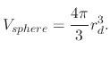
Using the equation for the volume of a sphere, the relationship between volume and radius is established as
.
Using the equation for the volume of a sphere, the relationship between volume and radius is established as
 |
(250) |
Therefore, when the volume is evenly distributed, the effect on the radius will be
 . Initially, it might be counter-intuitive
to note the inverse relationship since
. Initially, it might be counter-intuitive
to note the inverse relationship since
 . However, when a volume of
  is distributed for a radius
  m, then
 |
(251) |
where  is the number fraction, resulting in
  . When the same volume is distributed for droplets of a radius
  m, then the calculation above
leads to the number fraction
m, then the calculation above
leads to the number fraction
 , which is 8 times less, or
 times less.
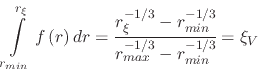
Now we know that the radius distribution should follow the equation
 |
(252) |
where  is a normalization constant which must be found,
  is the randomly distributed radius, and
  is the radius relating
and to an even volume distribution
is the radius relating
and to an even volume distribution
![$ \xi_V\in\left[0,1\right]$](img952.png) from (B.1)
from (B.1)
![$\displaystyle r_{\xi}=\cfrac{C}{\left[\left(r_{max}-r_{min}\right)\xi_V+r_{min}\right]^{3}}.$](img953.png) |
(253) |
Inverting (B.5) to solve for  allows to find the CPD function

![$\displaystyle \Phi\left(r_{\xi}\right)=\xi_V=\cfrac{1}{r_{max}-r_{min}}\left[\left(\cfrac{C}{r_{\xi}}\right)^{1\slash3}-r_{min}\right].$](img956.png) |
(254) |
The derivative of (B.6) gives the PDF
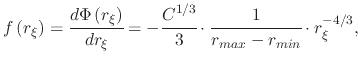 |
(255) |
where it can be noted that the last term from (B.6) has disappeared. The only non-constant term in (B.7) is
 , therefore a replacement constant, which will be the new normalization constant is introduced for simplicity
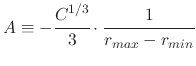 |
(256) |
and (B.7) can be rewritten to
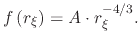 |
(257) |
Using the PDF from (B.9), we can now proceed to find the normalized distribution , but first the normalization constant  must be
found by integrating (B.9) with respect to from to and equating the integral to 1
must be
found by integrating (B.9) with respect to from to and equating the integral to 1
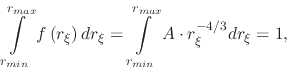 |
(258) |
which can be solved to
![$\displaystyle -3A\left[\left(\cfrac{1}{r_{max}}\right)^{1\slash3}-\left(\cfrac{1}{r_{min}}\right)^{1\slash3}\right]=1,$](img962.png) |
(259) |
giving the normalization constant
![$\displaystyle A=-\cfrac{1}{3\left[r_{max}^{-1\slash3}-r_{min}^{-1\slash3}\right]}$](img963.png) |
(260) |
and the normalized PDF
![$\displaystyle f\left(r_{d}\right)=-\cfrac{1}{3\left[r_{max}^{-1\slash3}-r_{min}^{-1\slash3}\right]}\cdot r_{d}^{-4\slash3}.$](img964.png) |
(261) |
Now one can integrate the normalized PDF from to to find the CPD
 |
(262) |
and invert the CPD to find the quantile function and solve for
![$\displaystyle r_{\xi}=\left\{ \xi_V\cdot\left[\left(r_{max}\right)^{-1\slash3}-...
...{min}\right)^{-1\slash3}\right]+\left(r_{min}\right)^{-1\slash3}\right\} ^{-3},$](img966.png) |
(263) |
which gives the equation for the radius distribution between and when the volume number fraction
is evenly distributed and
.
L. Filipovic: Topography Simulation of Novel Processing Techniques