A.2 Transport under a Velocity- and Displacement-Dependent Acceleration

When the acceleration of a droplet also depends on the droplet's position in a simulation environment, or the displacement from its original position, such as is the case with the application of an electric force to a droplet's transport, the total force experienced by a droplet becomes

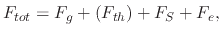$$F_{tot}=F_{g}+\left(F_{th}\right)+F_{S}+F_{e},$$ (228)

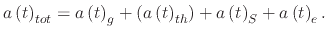
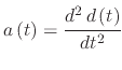
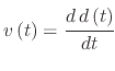
where $F_e$ is the electric force and the acceleration becomes

$$a\left(t\right)_{tot}=a\left(t\right)_{g}+\left(a\left(t\right)_{th}\right)+a\left(t\right)_{S}+a\left(t\right)_{e}.$$ (229)

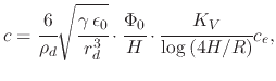
Acceleration due to the applied electric field is modeled as a linear displacement-dependent acceleration from (5.28)

$$c=\cfrac{6}{\rho_{d}}\sqrt{\cfrac{\gamma\,\epsilon_{0}}{r_{d}^{3}}}\cdot\cfrac{\Phi_{0}}{H}\cdot\cfrac{K_{V}}{\log\left(4H\slash R\right)}c_{e},$$ (230)

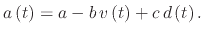
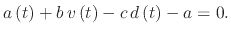
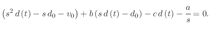
while acceleration due to gravity and the Stokes component of the acceleration remain the same from Section A.1. Therefore, the following equation must be solved to find the droplet displacement after time $t$

$$a\left(t\right)=a-b\,v\left(t\right)+c\,d\left(t\right).$$ (231)

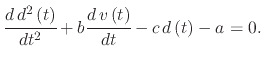
The equation can be re-written into a standard quadratic form, which is easier to solve

$$a\left(t\right)+b\,v\left(t\right)-c\,d\left(t\right)-a=0.$$ (232)

Noting that $a\left(t\right)=\cfrac{d^{2}\,d\left(t\right)}{dt^{2}}$, $v\left(t\right)=\cfrac{d\,d\left(t\right)}{dt}$, and $d\left(t\right)$ is the displacement.

$$\cfrac{d\,d^{2}\left(t\right)}{dt^{2}}+b\cfrac{d\,v\left(t\right)}{dt}-c\,d\left(t\right)-a=0.$$ (233)

Using the Laplace method for solving differential equations, the characteristic equation, (A.26) can be re-written using $s$ to depict a derivation step and $r_i$ to depict the roots of equations. Assuming the initial velocity $v_0$ and initial displacement $d_0$, (A.26) becomes

$$\left(s^{2}\, d\left(t\right)-s\, d_{0}-v_{0}\right)+b\left(s\, d\left(t\right)-d_{0}\right)-c\, d\left(t\right)-\cfrac{a}{s}=0.$$ (234)

Multiplying by $s$ gives

$$s^{3}\, d\left(t\right)-s^{2}\, d_{0}-s\, v_{0}+s^{2}\, b\, d\left(t\right)-s\, b\, d_{0}-s\, c\, d\left(t\right)-a=0.$$ (235)

Isolating for $d\left(t\right)$ gives

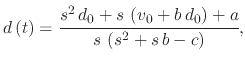$$d\left(t\right)=\cfrac{s^{2}\, d_{0}+s\,\left(v_{0}+b\, d_{0}\right)+a}{s\,\left(s^{2}+s\, b-c\right)},$$ (236)

which is then split according to the numerator's power of $s$ using partial fractional decomposition

$$\begin{array}{rccccc} d\left(t\right)= & \underbrace{\cfrac{s... ...stem 1} & & \textrm{System 2} & & \textrm{System 3} \end{array}$$ (237)

The roots of the equation can be found by finding $s$ values for which (A.30) is invalid, or infinity. These roots are

$$r_{1}=\cfrac{-b+\sqrt{b^{2}+4c}}{2},\quad r_{2}=\cfrac{-b-\sqrt{b^{2}+4c}}{2},\quad r_{3}=0.$$ (238)

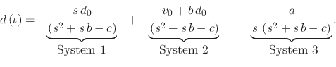
In order to find the final equation for the displacement $d\left(t\right)$, a solution to each system in (A.30) must be found and added together

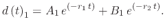
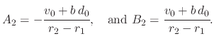
• System 1
  System 1 is set up such that the two roots are separated

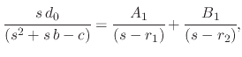  $$\cfrac{s\, d_{0}}{\left(s^{2}+s\, b-c\right)}=\cfrac{A_{1}}{\left(s-r_{1}\right)}+\cfrac{B_{1}}{\left(s-r_{2}\right)},$$ (239)

  
  
  where $A_1$ and $B_1$ are parameters to solve the displacement due to System 1

  $$d\left(t\right)_{1}=A_{1}\,e^{(-r_{1}\,t)}+B_{1}\,e^{(-r_{2}\,t)}.$$ (240)

  
  
  $A_1$ and $B_1$ are found using (A.32)

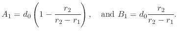  $$A_{1}=d_{0}\left(1-\cfrac{r_{2}}{r_{2}-r_{1}}\right),\quad\textrm{and }B_{1}=d_{0}\cfrac{r_{2}}{r_{2}-r_{1}}.$$ (241)

  
  

• System 2
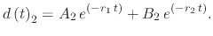
  Similar to System 1, System 2 is set up, separating the effects from the two roots

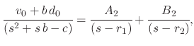  $$\cfrac{v_{0}+b\, d_{0}}{\left(s^{2}+s\, b-c\right)}=\cfrac{A_{2}}{\left(s-r_{1}\right)}+\cfrac{B_{2}}{\left(s-r_{2}\right)},$$ (242)

  
  
  where $A_2$ and $B_2$ are parameters to solve the displacement due to System 2

  $$d\left(t\right)_{2}=A_{2}\,e^{(-r_{1}\,t)}+B_{2}\,e^{(-r_{2}\,t)}.$$ (243)

  
  
  $A_2$ and $B_2$ are found using (A.35)

  $$A_{2}=-\cfrac{v_{0}+b\, d_{0}}{r_{2}-r_{1}},\quad\textrm{and }B_{2}=\cfrac{v_{0}+b\, d_{0}}{r_{2}-r_{1}}.$$ (244)

  
  

• System 3
  System 3 has an additional root involvement from the presence of $s$ in the denominator, so the system is set up as

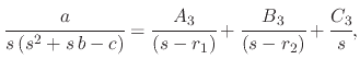  $$\cfrac{a}{s\left(s^{2}+s\, b-c\right)}=\cfrac{A_{3}}{\left(s-r_{1}\right)}+\cfrac{B_{3}}{\left(s-r_{2}\right)}+\cfrac{C_{3}}{s},$$ (245)

  
  
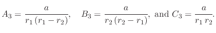
  where $A_3$, $B_3$, and $C_3$ are parameters to solve the displacement due to System 3

  $$d\left(t\right)_{3}=A_{3}\,e^{(-r_{1}\,t)}+B_{3}\,e^{(-r_{2}\,t)}+C_{3}.$$ (246)

  
  
  $A_3$, $B_3$, and $C_3$ are found using (A.38)

  $$A_{3}=\cfrac{a}{r_{1}\left(r_{1}-r_{2}\right)},\quad B_{3}=\cfrac{a}{r_{2}\left(r_{2}-r_{1}\right)},\textrm{ and } C_{3}=\cfrac{a}{r_{1}\, r_{2}}.$$ (247)

  
  

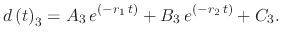
After combining all three systems, the equation which governs the displacement at time $t$ due to velocity and displacement-dependent acceleration is given by

$$d\left(t\right)=\left(A_{1}+A_{2}+A_{3}\right)\,e^{-r_{1}\, t}+\left(B_{1}+B_{2}+B_{3}\right)\,e^{-r_{2}\, t}+C_{3}.$$ (248)

It should be noted that, if the initial displacement is set to 0, then $A_1=B_1=0$. Similarly, if the initial velocity is also set to 0, then $A_2=B_2=0$, significantly reducing the complexity of the problem.