A.1 Original FOWLER-NORDHEIM Formula

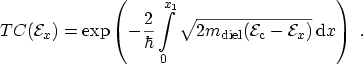
The original FOWLER-NORDHEIM formula assumes a triangular shape of the energy barrier. This is motivated by the fact that only tunneling at strong electric fields was studied. The WKB-approximation (3.55) for the transmission coefficient reads

$$TC({\mathcal{E}}_x)=\exp\left(-\frac{2}{\hbar} \int_0^{x_1}\sqrt{... ...mathcal{E}}_\mathrm{c}}-{\mathcal{E}}_x)}\,\ensuremath {\mathrm{d}}x\right) \ .$$

The classical turning point $x_1$ is (see the left part of Fig. A.1)

$$x_1 = \frac{\ensuremath{{\mathcal{E}}_\mathrm{f,1}}+ \ensuremath ... ..._1 - {\mathcal{E}}_x}{\ensuremath {\mathrm{q}}\ensuremath{E_\mathrm{diel}}} \ ,$$

and the dielectric conduction band edge for a triangular barrier

$$\ensuremath {{\mathcal{E}}_\mathrm{c}}(x)=\ensuremath{{\mathcal{E... ... {\mathrm{q}}\Phi_1 - \ensuremath {\mathrm{q}}\ensuremath{E_\mathrm{diel}}x \ ,$$

where the electric field in the dielectric $\ensuremath{E_\mathrm{diel}}$ is caused by the different Fermi levels and the work function difference $\Delta \ensuremath{\Phi_\mathrm{W}}$:

$$\ensuremath{E_\mathrm{diel}}= \frac{\ensuremath{{\mathcal{E}}_\ma... ...ath{\Phi_\mathrm{W}}}{\ensuremath {\mathrm{q}}\ensuremath{t_\mathrm{diel}}} \ .$$

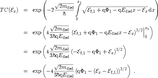
The third approximation is to assume equal materials for both electrodes, so that $\Delta \ensuremath{\Phi_\mathrm{W}}= 0$. The WKB-based transmission coefficient can then be applied and yields

$$\renewcommand {\arraystretch }{2.8} \begin{array}{rcl} TC({\mathc... ... - \ensuremath{{\mathcal{E}}_\mathrm{f,1}})\right)^{3/2}\right) \ . \end{array}$$ (A.6)

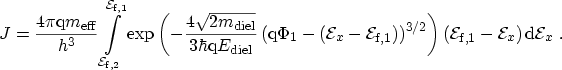
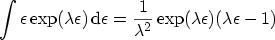
Using this expression in (A.5) the current density becomes

$$J=\frac{4\pi \ensuremath {\mathrm{q}}\ensuremath{m_\mathrm{eff}}}... ...}}_\mathrm{f,1}}-{\mathcal{E}}_x) \,\ensuremath {\mathrm{d}}{\mathcal{E}}_x \ .$$ (A.7)

This integral cannot be solved analytically. Hence, the fourth approximation is to expand the square root into a first order TAYLOR^A.1series around $\Phi_1$:

$$\left( \ensuremath {\mathrm{q}}\Phi_1 - ({\mathcal{E}}_x - \ensur... ...uremath{{\mathcal{E}}_\mathrm{f,1}}) (\ensuremath {\mathrm{q}}\Phi_1)^{1/2} \ .$$ (A.8)

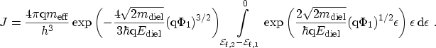
Inserting this expression into (A.7) and setting $\epsilon = {\mathcal{E}}_x - \ensuremath{{\mathcal{E}}_\mathrm{f,1}}$ yields

$$J=\frac{4\pi \ensuremath {\mathrm{q}}\ensuremath{m_\mathrm{eff}}}... ...}}\Phi_1)^{1/2} \epsilon\right) \epsilon \,\ensuremath {\mathrm{d}}\epsilon \ .$$ (A.9)

With

$$\int\epsilon \exp(\lambda \epsilon) \, \ensuremath {\mathrm{d}}\epsilon = \frac{1}{\lambda ^2} \exp(\lambda \epsilon) (\lambda \epsilon -1)$$ (A.10)

and

$$\begin{array}{cp{1cm}c} a=-\displaystyle\frac{4\sqrt{2\ensure... ...m{diel}}} (\ensuremath {\mathrm{q}}\Phi_1)^{1/2}\ , \end{array}$$ (A.11)

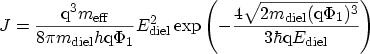
the current density becomes

$$J = \frac{4\pi \ensuremath {\mathrm{q}}\ensuremath{m_\mathrm{eff}... ...athcal{E}}_\mathrm{f,2}}- \ensuremath{{\mathcal{E}}_\mathrm{f,1}}) -1\right)\ .$$ (A.12)

The fifth assumption is now that $\ensuremath{{\mathcal{E}}_\mathrm{f,1}} \gg \ensuremath{{\mathcal{E}}_\mathrm{f,2}}$, leading to

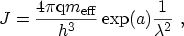$$J=\frac {4\pi \ensuremath {\mathrm{q}}\ensuremath{m_\mathrm{eff}}} {h^3} \exp(a) \frac{1}{\lambda^2}\ ,$$ (A.13)

or

$$J= \frac {\ensuremath {\mathrm{q}}^3\ensuremath{m_\mathrm{eff}}} ... ...hi_1)^3}} {3\hbar \ensuremath {\mathrm{q}}\ensuremath{E_\mathrm{diel}}} \right)$$ (A.14)

which is the equation commonly known as the FOWLER-NORDHEIM formula. Note that there is a difference between the effective electron mass in the electrode ( $m_\mathrm{eff}$) and the effective electron mass in the dielectric ( $m_\mathrm{diel}$).

A. Gehring: Simulation of Tunneling in Semiconductor Devices