![∑ ∫
1 i τi1(k1) ⋅ f(E )(1 - f (E))dk1
------= --------∑---∫------------------,
τm[τs] i f(E )dk1](diss_htm181x.png)
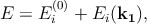
The spin relaxation times for all the individual components are evaluated by thermal averaging [71, 53, 69] as
|
| (4.12) |
where
 | (4.13) |


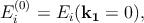
![f (E ) = [-------1-------].
1 + exp (E-EF-)
KBT](diss_htm186x.png) | (4.14) |
Here,
where
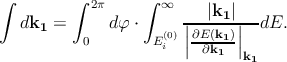
The spin-flip rate can be written as [55]
![1 4π ∑ ∫ 2π 1 ℏ4 |k |
----------= ------- dφ ⋅ π△2L2 ⋅ -2----------⋅---2 ⋅|---2--|
τi,s,SR(k1 ) ℏ(2π)2 j=1,2 0 ϵij|k2 - k1| 4m l ||∂E∂(kk2)||
( ) 2
[( dΨik1σ) *(dΨjk2 -σ)]2 - |k2 - k1|2L2
⋅ ------- -------- t⋅ exp --------------
dz dz z=± 2 4
⋅ θ(E (k ) - E(0)).
j 2 j](diss_htm189x.png) | (4.16) |
Here,
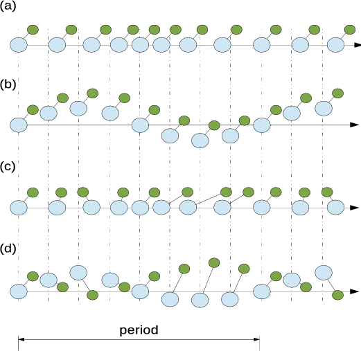
Phonons are the lattice vibrations, but those can be imagined as particles which carry vibrational energy in a similar manner to photons, i.e. they are discrete and quantized [117]. The energy of a phonon is characterized by its own intrinsic frequency. In a lattice with a basis of more than one atom in the primitive cell (which may or may not be different), the allowed frequencies of a propagating wave can be split into an upper branch known as the optical branch, and a lower branch called the acoustical branch. Acoustic phonons are coherent movements of atoms of the lattice out of their equilibrium positions. In contrast for optic phonons, the center of mass of the cell during oscillations does not move [117, 128, 155] (i.e. one atom moving to the left, and its neighbour to the right). The nature of the vibrations are sketched in Figure 4.9. The acoustic branch has its name because it gives rise to long wavelength vibrations, and the speed of its propagation is the speed of a sound wave in the lattice. The optical branch is a higher energy vibration, and one can excite these modes with the electromagnetic radiation [117]. For both of acoustic and optical modes, the vibration is restricted to the direction of propagation in the longitudinal mode, whereas in the transversal mode the vibration occurs in the perpendicular planes.
In the three-dimensional lattice system the number of optical modes for the
primitive cell that contains
In the analysis of intrasubband electron-phonon scattering, the explicit forms of the polarization vectors of phonons are needed. Following [156, 53] the phonons polarization vectors can be written as
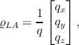 | (4.17) |
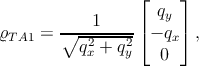 | (4.18) |
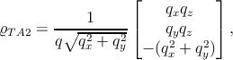 | (4.19) |
where  is related to the momentum transfer in the
scattering [53].
is related to the momentum transfer in the
scattering [53].
The formulation for the transition rate from one energy eigenstate of a
quantum system into the other energy eigenstates in a continuum is given by
Fermi’s golden rule [157]. The electron-phonon mediated momentum and the spin
relaxation rates, where
 | (4.20) |
where
The spin relaxation rate for the wave vector
![1 4πK T ∑ ∫ 2πdφ ∫ ∞ dq |k |
---------= ----B--- --- ---z--|---2-|-
τi,AC(k1) ℏρ ν2 j 0 2π -∞ (2π )2||∂E∂(kk2)||
| | 2
[ ||∂E(k2)||f(E (k2))]
⋅ 1 - |-∂k2-|----------
||∂E(k1)||f(E (k ))
∂k1 1 ∫
∑ ||qα1 t † ||2
⋅ |---ϱα2(q )Dα1α2 dzΨ jk2-σ(z)exp (- iqzz)Ψik1σ(z)|
α1α2 q 0
(0)
⋅ θ(Ej (k2 ) - Ej ).](diss_htm196x.png) | (4.21) |
Here, the momentum transfer vector
By applying Fubini’s theorem the modulus in the above equation can be replaced by a repeated integral,
![1 4πK T ∑ ∫ 2πdφ ∫ ∞ dq |k |
---------= ----B--- --- ----z-|---2--|
τi,AC(k1 ) ℏ ρν2 j 0 2 π -∞ (2π )2||∂E∂(kk2)||
| | 2
[ ||∂E(k2)||f(E (k2))]
⋅ 1 - |-∂k2-|----------
||∂E(k1)||f(E (k ))
∫ ∫ ∂k1 1
t t ′[ † AC ]*
⋅ dz dz ψjk2-σ(z)M ψik1σ(z)
[ 0 0 ]
⋅ ψ † (z′)M ACψik1σ(z′) LAC exp(- iqz|z - z ′|)
jk2- σ
⋅ θ(Ej (k2) - E(j0)).](diss_htm197x.png) | (4.22) |
![1 4 πK T ∑ ∫ 2π dφ 1 |k |
--------- = -----B-- ---------|--2--|-
τi,AC (k1) ℏρν2 j 0 2π (2π)2 ||∂E∂(kk2)||
| | 2
[ ||∂E(k2)||f(E (k2 ))]
⋅ 1 - |--∂k2--|---------
||∂E(k1)||f(E (k ))
∫ ∫ ∂k1 1
t t ′[ † AC ]*
⋅ dz dz ψ jk2-σ (z )M ψik1σ(z)
[0 0 ] ∫ ∞
⋅ ψ† (z′)M AC ψ (z′) dq L exp(- iq|z - z′|)dz′
jk2-σ ik1σ -∞ z AC z
(0)
⋅ θ(Ej(k2 ) - E j ).](diss_htm198x.png) | (4.23) |
The g-process describes the electron intervalley scattering between opposite
valleys, which includes only the [001] valley pair in the Brillouin zone. The
f-process involves scattering between valleys that reside on perpendicular axes,
which will be treated later. For intervalley scattering [53],
![∫ [ † ] [ † ]
dz′ ψjk2-σ(z′)M AC ψik1σ(z′) δ(z - z′) = ψjk2-σ(z)M AC ψik1σ(z) .](diss_htm199x.png) | (4.24) |
This simplifies Equation 4.23 to
![1 4πK T ∑ ∫ 2πd φ 1 |k |
---------= ----B2--- --- ⋅----2-|---2-|-
τi,LA(k1 ) ℏρνLA j 0 2 π (2π) ||∂E∂(kk2)||
| | 2
[ ||∂E(k2)||f (E (k2))]
⋅ 1 - |-∂k2-|----------
||∂E(k1)||f (E (k1))
∫ ∂k1
t [ † AC ]*[ † AC ]
⋅ 2π dz ψjk2-σ(z)M ψik1σ(z) ψ jk2-σ (z )M ψik1σ(z)
0
⋅ θ(Ej (k2) - Ej(0)).](diss_htm200x.png) | (4.25) |
Here,  ,
,
![[ ]
′ MZZ MSO
M = M †SO MZZ ,](diss_htm202x.png) | (4.26) |
![[ ]
Ξ 0
MZZ = 0 Ξ ,](diss_htm203x.png) | (4.27) |
![[ ]
0 DSO (ry - irx)
MSO = DSO (- ry - irx) 0 ,](diss_htm204x.png) | (4.28) |
where (
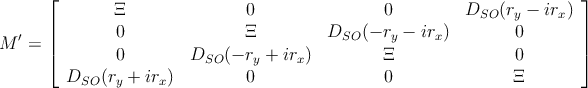 | (4.29) |
Intrasubband transitions are important for the contributions determined by the
shear deformation potential. The term
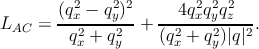 | (4.30) |
Applying the theory of residues with
![∫ ∫
∞ q2z exp(--iqz|z---z′|) ∞ q2z exp-(- iqz|z --z′|)
dqz (Q2 + q2)2 = dqz (iQ - q )2(iQ + q )2
-∞ z -∞ [( 2 z z ′ ) ]
= - 2 πi -d--qz exp-(- iqz|z --z|)
dqz (iQ - qz)2 qz=-iQ
′
= π-1 --Q|z---z-|exp(- Q |z - z′|).
2 Q](diss_htm207x.png) | (4.31) |
The matrix
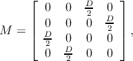 | (4.32) |
where
Following Equation 4.23 the intrasubband transversal acoustic phonons is
![∑ ∫ 2π
---1-----= 4πKBT--- dφ- ⋅--1---||k2|-|-
τi,TA(k1) ℏρν2TA j 0 2π (2π)2 ||∂E(k2)||
| | ∂k2
[ ||∂E(k2)||f(E (k ))]
⋅ 1 - |-∂k2-|------2---
|∂E(k1)|
| ∂k1 |f(E (k1))
∫ t ∫ t ∘ ------- π
⋅ dz dz′exp(- q2x + q2y|z - z ′|) ⋅-
[0 0 ] [ 2 ]
⋅ Ψ † (z)M Ψ (z )* Ψ † (z)M Ψ (z)
[ jk2-σ ik1σ jk2-]σ ik1σ
4q2q2(1 - |z - z′|∘q2-+--q2)
⋅ --x-y---∘-----------x----y- ⋅ θ(Ej(k2) - E (0j)).
( q2x + q2y)3](diss_htm209x.png) | (4.33) |
Here,  is the transversal phonon velocity, and
  is the silicon
density [158].
is the silicon
density [158].
The term
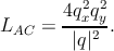 | (4.34) |
Applying the theory of residues with
![∫ ∞ exp(- iqz|z - z′|) ∫ ∞ exp (- iqz|z - z′|)
dqz------2----22----= dqz ---------2--------2-
- ∞ (Q + qz) -∞ (iQ - qz)(iQ + qz)
[(-d--exp(--iqz|z---z′|)-) ]
= - 2 πi dq (iQ - q )2 q= -iQ
′z z z
= π-Q|z---z-| +-1-exp(- Q |z - z′|).
2 Q3](diss_htm213x.png) | (4.35) |
The matrix
![∫
----1---- 4-πKBT--∑ 2π dφ- --1--- --|k2-|--
τi,LA (k1) = ℏρ ν2 2π ⋅ (2π)2 ⋅ ||∂E(k2)||
LA j 0 | ∂k2 |
[ ||∂E (k2)|| ]
|--∂k2-|f(E (k2))
⋅ 1 - ||∂E-(k-)||---------
|--∂k11-|f(E (k1))
∫ t ∫ t ∘ -------
⋅ dz dz ′exp (- q2+ q2|z - z′|) π-
0 0 x y 2
[ † ]*[ † ]
⋅ Ψ jk2- σ(z )M Ψik1σ(z) Ψ jk2- σ(z)M Ψik1σ(z)
2 2 [∘ ------- ]
⋅--4qxqy--- q2 + q2|z - z′| + 1 θ(E (k ) - E (0)).
(q2x + q2y)32 x y j 2 j](diss_htm214x.png) | (4.36) |
When both the surface roughness and the acoustic phonon mediated components are calculated, the total spin lifetime is calculated by the Matthiessen rule.