5.1 Semi-Classical Model of Charge Transport
5.1.1 Poisson’s Equation
The Poisson equation correlates the electrostatic potential V to a given charge
distribution  . If the permittivity tensor is expressed as
  , one can write the
Poisson equation as
, one can write the
Poisson equation as
 | (5.1) |
The charge distribution can be expressed as  = q(p - n + C), where n (p)
represents the electron (hole) concentration per unit volume, q is the fundamental
charge unit, and the concentrations of ionized impurities and the dopant are
added up as the fixed charge concentration C. These fixed charges can originate
from charged impurities of donor (ND) and acceptor (NA) type and from trapped
electrons (C1) and holes (C2)
= q(p - n + C), where n (p)
represents the electron (hole) concentration per unit volume, q is the fundamental
charge unit, and the concentrations of ionized impurities and the dopant are
added up as the fixed charge concentration C. These fixed charges can originate
from charged impurities of donor (ND) and acceptor (NA) type and from trapped
electrons (C1) and holes (C2)
 | (5.2) |
The electric field (Ẽ) is related to V by
 | (5.3) |
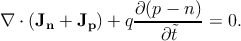
5.1.2 Continuity Equations
The charge transport model is derived from the continuity equation which takes
care of mass conservation (time is represented by  )
)
 | (5.4) |
The total current density is J. One can decompose the contributions of the
current J = Jn + Jp, where Jn (Jp) denotes the electron (hole) current density.
Assuming all immobile charges as fixed with respect to time,  = q
= q as
as
 = 0. Then, the continuity equation (Equation 5.4) can be separated into an
electron and a hole related parts,
= 0. Then, the continuity equation (Equation 5.4) can be separated into an
electron and a hole related parts,
 | (5.5) |
This step enables to write the electron and hole related contributions as two
independent equations,
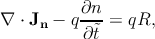 | (5.6a) |
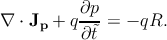 | (5.6b) |
where the net generation-recombination rate is represented as R.
5.1.3 Drift-Diffusion Equations
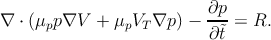
As the Poisson equation (Equation 5.1) and the two continuity equations
(Equation 5.6a and Equation 5.6b) involve five unknown quantities (viz. V , n, p,
Jn, and Jp), one needs two more conditions to make the equation system
complete. Now, there are two major effects which lead to current flow in
semiconductors (e.g. silicon). First, the drift of charged carriers due to the
influence of an electric field, and second, the diffusion current due to a
concentration gradient of the carriers. It is hereby mentioned that the
drift-diffusion model considers the temperature to be constant throughout the
device [179], both for the charge carriers and the lattice.
The charged carriers in a semiconductor subjected to an electric field are
accelerated and acquire a certain drift velocity. The orientation depends on the
charge state, holes are accelerated in direction of the electric field and electrons in
the opposite direction. The magnitude of the drift velocity depends on the
probability of scattering events. At low impurity concentration, the carriers
mainly collide with the crystal lattice. When the impurity concentration is
increased the collision probability with the charged dopants through Coulomb
interaction becomes more and more likely, thus reducing the drift velocity with
increasing doping concentration [180].
The drift component is expressed using the concept of carrier mobility, which
is the proportionality factor between the electric field strength (Ẽ) and
the average carrier velocity. If one denotes μn (μp) as the electron (hole)
mobility (assumed isotropic in the channel under investigation), in the
low electric field range one can write the corresponding average carrier
velocities as vn = -μnẼ and vp = μpẼ. Then the drift current density for the
electrons and the holes can be expressed as JDrift
n = -qnvn = qnμnẼ and
JDrift
p = qpvp = qpμpẼ. The signs are justified as electrons (holes) move
against (with) the field direction. One can express the conductivities as
σn = qnμn for the electrons and σp = qpμp for the holes, then JDrift
n = σnẼ and
JDrift
p = σpẼ.
A concentration gradient of carriers leads to carrier diffusion. This is because
of their random thermal motion which is more probable in the direction of
the lower concentration. The electron current contribution due to the
concentration gradient is written as JDiffusion
n = qDn∇n and the hole current as
JDiffusion
p = -qDp∇p, where Dn and Dp are the diffusion coefficients for electrons
and holes. For the non-degenerate semiconductors and in thermal equilibrium, one
can relate the diffusion coefficient with the mobility by using Einstein’s relation
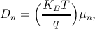 | (5.7a) |
 | (5.7b) |
where KB is the Boltzmann’s constant, and T is the temperature. The thermal
voltage (VT ) is described as
 | (5.8) |
Thus, the diffusion coefficients can be written as Dn = μnVT and Dp = μpVT .
Here, the non-degenerate semiconductors are defined as semiconductors for which
the Fermi energy is at least 3KBT away from both the conduction and the valence
band edges [117, 179]. One can assume the considered semiconductor to
be lightly doped and thus non-degenerate, as it is the case in spintronic
applications [173]. However, when the doping becomes very high, the Fermi
level rises more and more towards the conduction band and the transport
becomes degenerate. In such a case, the transport equations must be
expressed in the language of chemical potentials of the carriers instead of their
concentrations [173, 181].
Combining the current contributions of the drift and the diffusion effect one
gets
 | (5.9a) |
 | (5.9b) |
By inserting Equation 5.9a into Equation 5.6a and Equation 5.9b into
Equation 5.6b one obtains
 | (5.10a) |
 | (5.10b) |
From the equations Equation 5.1, Equation 5.10a, and Equation 5.10b, one can
obtain the unknown parameters n, p, and V . Despite the clear limitations for the
description of state-of-the-art devices, these set of equations are still widely
used in TCAD applications due to their least qualitative results and their
computational inexpensiveness.
5.1.4 Quasi-Fermi Levels
The thermal equilibrium does not demand a position-independent potential. For
instance
denoting the conduction band edge energy EC, the valence band edge energy
EV , and the intrinsic Fermi level energy Ei, respectively. Treating the situation
away from thermal equilibrium complicates the matter. One can reformulate
Equation 5.9a with Equation 5.3 as
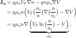 | (5.12) |
where ni is the intrinsic carrier concentration. This shows that the drift and the
diffusive contribution can be merged into one quantity. This quantity can
be related to the quasi-Fermi level as follows [182] -qϕn = EF,n - Ei,0.
Therefore, the current depends on the gradient of the quasi-Fermi levels
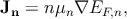 | (5.13a) |
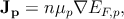 | (5.13b) |
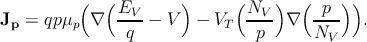
The drift-diffusion current relations consider position dependent band edge
energies, EC(r) for the conduction band and EV (r) for the valence band, and
position dependent effective masses, which are included in the effective density of
states NC for the electrons and NV for the holes, can be expressed as [183, 184]
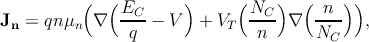 | (5.14a) |
 | (5.14b) |