2.1 Band Structure Calculation Methods in Semiconductors

As the study of semiconductor properties are a fundamental part of the solid-state physics research, the investigation of the band structure via computational means are of great importance. Modern methods to calculate the electronic band structure are sophisticated enough to describe the subband behavior of semiconductors. However, commonly used methods demand the implementation of complex algorithms and a huge amount of computational power.

Both the empirical and ab-initio methods are utilized to evaluate the band structure of solids. The empirical methods rely on using a small number of adjustable parameters to obtain a fit to certain known features of the bulk band structure, whereas the ab-initio methods determine the band structure from the first principles and do not need any experimental input. Hence, a first principle approach typically involves heavy amount of computational effort, whereas the empirical methods do not [114].

Methods to calculate the band structure of a solid by using first principles can be divided into several groups. The density functional theory (DFT) is widely used to investigate the electronic structures i.e. principally the ground state of many-body systems, in particular atoms, molecules, and condensed phases [115]. The non-equilibrium Greens function (NEGF) function provides a formalism for the description of transport phenomena of nanoscale devices [116]. Now-a-days, these are extensively used to study the new materials [114]. The most popular empirical methods are based on either pseudopotential or tight-binding methods. On the other hand, by using the perturbative k ⋅ p method (also a semi-empirical method) one can obtain analytical expressions for the band dispersion and the effective masses averting heavy numerical analysis [72]. In the following section, several methods and their key properties are described in brief.

2.1.1 Nearly-Free Electron Approximation

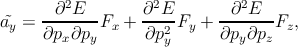
In the nearly-free electron approximation, interactions between electrons are completely ignored. This approximation allows the use of Bloch’s Theorem, which states that electrons in a periodic potential have wave functions and energies which are periodic in wave vector up to a constant phase shift between neighboring reciprocal lattice vectors [117]

(2.1)

where the function u_n,k(r) is periodic over the crystal lattice

(2.2)

with R as the periodicity. These plane wave solutions have an energy of E(k) = (m_e is the electron rest mass). The electron wave function can be approximated by u_n,k(r) = , where Ω_r is the volume occupied by the electron. This over-simplified method works well in the materials where the lattice constant is low (e.g. alkali metals like Na, K, Al and those have one electron in the primitive cell), and the lattice potential is only a small perturbation to the electron sea.

2.1.2 Tight-Binding Approximation

The tight-binding (TB) method uses the atomic orbitals as basis for the wave functions [118]. The electrons are assumed to be tightly bound to their atoms and they must have limited interaction with states and potentials of surrounding atoms of the solid. The crystal potential is strong. As a result the wave function of the electron will be rather similar to the atomic orbital of the bound atom to which it belongs. Any correction from the initial system Hamiltonian to the atomic potential are assumed small. Therefore, this can be considered as the opposite extreme to the nearly free electron approximation. Generally this method is good at describing the inner electronic shells of the atoms. Although the TB approximation neglects the electron-electron interactions, one can still reproduce accurately the band structure of many solids including metals by using this method.

The wave function is constructed from the valence orbitals of all of the atoms in a primitive cell of the crystal. Thus, the single electron wave function can be represented as a linear combination of the atomic orbitals

(2.3)

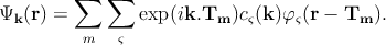
Here, the atoms are characterized by the atomic orbitals φ_ς(r) (ς refers to the atomic energy level). This atomic orbital is the eigenfunctions of the Hamiltonian of a single isolated atom. T_m specifies the position of the m^th atom, and the function φ_ς(r - T_m) represents the atomic orbital centered around the m^th atom. The coefficients c_ς(k) are found from the Schrödinger equation. It can be shown that Ψ_k(r) in Equation 2.3 is a Bloch function which satisfies the necessary requirement,

(2.4)

where T is the real space crystal translation vector. Now by substituting this equation into the Schrödinger equation, one can form a set of linear equations with respect to the coefficient c_ς(k). The number of equations is equal to the number of considered orbitals in an atom, thus the solution represents the respective energy bands. The function Ψ_k(r) therefore satisfies both the requirement of the Bloch theorem and the assumptions in the TB model. It can be used to calculate the energy of a band via E(k) =  [118], where H is the Hamiltonian of the electron.

Several semi-empirical TB models are available in literature depending on different number of orbitals and order of neighbors included [119, 120, 121, 122, 123]. This method can also be easily adapted to strained nanostructures [123].

2.1.3 Cellular Method

The cellular method was the earliest method employed in the band structure calculations by Wigner and Seitz (WS) [124]. In this method, one divides the crystal into several unit cells (WS cell), and each atom is supposed to center at the middle of its cell. The electron, when in a particular cell, is assumed to be only influenced by the ionic potential in that cell. In order to ensure that the function Ψ_k satisfies the Bloch form as described earlier, u_k is periodic, i.e. it is same on the opposite faces of the cell under inspection. Since a WS cell usually has a complicated structure, the use of boundary conditions in a direct way is almost impossible. To avoid this difficulty, only the simplest approximation can be applied: the cell is replaced by a WS sphere with the same volume as the WS cell. This simplifies the problem to such an extent that a solution is possible, although such an approximation can only describe s-type states.

2.1.4 Augmented-Plane Wave Method

The augmented-plane wave method was developed by Slater in 1937 [125]. APW begins with the assumption that the effective crystal potential is constant between the cores (muffin-tin like potential). Outside the core the wave function is a plane wave as the potential is constant, and inside the core the function is atom-like to be solved by the free-atom Schrödinger equation.

2.1.5 Pseudopotential Method

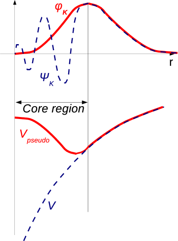
The pseudo-potential method differs from the above discussed methods by the manner in which the wave function is chosen [126]. The function which oscillates rapidly inside the core, but runs smoothly as a plane wave in the remainder of the open space of the WS cell, is sought for. This phenomenon is drawn in Figure 2.1.

One can write the expression for the wave function [127],

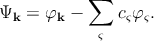(2.5)

where φ_k is a plane-wave like wave function (same as for the APW method), and φ_ς is an atomic wave function. In silicon which has an atomic number of fourteen (1s²2s²2p⁶3s²3p²), the summation over ς in Equation 2.5 is a sum over the core states 1s²2s²2p⁶ (i.e. all the occupied atomic shells). φ _k is the wave function of any of the outer core electrons, and φ_ς are the core wave functions. The coefficients c_ς are chosen such that the function Ψ_k is orthogonal to the core wave function φ_ς. By this orthogonality requirement, one can ensure that the outer electrons do not occupy the already filled atomic orbitals. Thus one can avoid violating the Pauli exclusion principle. The formulation of the Schrödinger equation with the pseudo-wave functions can be written as [127]

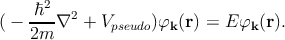(2.6)

Here, V_pseudo represents the pseudo-potential which cancels the crystal potential near the core region. The empirical pseudopotential method allows to reproduce all the characteristics including the band gap, spin-orbit split-off, the effective masses, the non-parabolicity parameters etc [72].

2.1.6 Perturbation Theory

Perturbation theory is widely used in mathematics to find an approximate solution to a problem, by starting from a known solution at a known position [72]. This theory is applicable when the problem can be formulated by adding a rather small term to the mathematical description of the exactly solvable problem. Thus, one can start with a system Hamiltonian associated with a known solution and then add an additional ’perturbing’ Hamiltonian which imposes a weak disturbance to the known system. On the other hand, one can divide the Hamiltonian representing the quantum state of a system into one bigger and one smaller part and apply the perturbation theory to deduce the approximated solution.

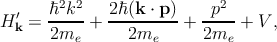
The k ⋅ p method is based on the perturbative approach and allows to obtain the analytical band structure close to a chosen point provided the eigenenergies and the eigenfunctions at that point are known. The expressions for the band dispersion and also the effective masses can be obtained by using this method [86, 128]. While the k ⋅ p theory has been frequently used to model the valence band of semiconductors, it can also be applied to model the impact of strain on the conduction band minimum [72]. One can write the one-electron Schrödinger equation as,

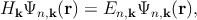(2.7)

where H_k is the system Hamiltonian

(2.8)

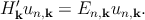
with n is the band index, k is the wave vector, m_e is the free electron mass, V is the potential energy, p is the electron momentum operator (p = -iℏ∇ with ℏ as the reduced Planck constant), E_n,k corresponds to the eigenenergy of the electron wave function Ψ_n,k. Due to the periodicity of the lattice potential, the Bloch theorem can be applied and the solution is of the form of Ψ_n,k = exp(ik.r)u_n,k.

If one now applies the Bloch wave function ansatz,

(2.9)

Again,

(2.10)

From these two identities, Equation 2.7 and Equation 2.8 involving the periodic function u_n,k rather than Ψ_n,k can be rewritten as

(2.11a)

(2.11b)

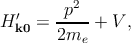
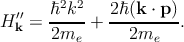
In any case, one can write this Hamiltonian as the sum of two terms H_k^′ = H _k0^′ + H _k^′′, where

(2.12a)

(2.12b)

Hence, the total Hamiltonian H_k^′ can be divided into an unperturbed part H_k0^′ with the eigenfunctions u _n,k0 at k = k₀, and a perturbative part H_k^′′.

2.1.7 Effective Mass Approximation

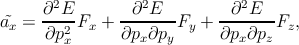
The mass of a free electron or the electronic rest mass can be expressed as m_e. When this electron is placed in a crystal lattice the situation changes, and the electron effective mass is the mass that it seems to have when responding to atomic forces. This effective mass must be interpreted as mass of the electron such that the classical energy formula E = holds. Considering the force acting on the electron is F, the acceleration ã of the electron can be represented as ã = . The expression for the velocity is v = where p represents the momentum of the electron. Since by definition F = , ã = = = F. By generalizing this equation for a three-dimensional model, one can write [129]

(2.13a)

(2.13b)

(2.13c)

The inverse of the position-dependent effective mass tensor can be expressed as (the momentum operator and the wave vector k are related by p = ℏk)

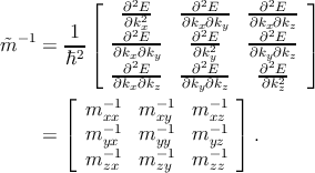(2.14)

The time-independent Schrödinger equation including is then expressed as [130]

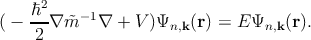(2.15)