3.1 Schrödinger-Poisson Solver
All NBTI models share the same challenge, namely to explain the correct
field acceleration and temperature activation of the  degradation.
These experimentally observed dependences must be traced back to the
physics in a MOSFET. The most frequently used charge trapping models
require the band diagram, the electric field across the insulator, and the
spatial distribution of the inversion charge carriers. This information can
easily be computed via a Poisson-solver (P-solver) or a Schrödinger-Poisson
solver (SP-solver) [129] if quantum mechanics are assumed to play a crucial
role.
degradation.
These experimentally observed dependences must be traced back to the
physics in a MOSFET. The most frequently used charge trapping models
require the band diagram, the electric field across the insulator, and the
spatial distribution of the inversion charge carriers. This information can
easily be computed via a Poisson-solver (P-solver) or a Schrödinger-Poisson
solver (SP-solver) [129] if quantum mechanics are assumed to play a crucial
role.
The electrostatics within a MOS device are described by the Poisson equation
where  denotes the electrical potential. The charge density is decomposed into the charge carrier densities of the electrons
  and holes
 and the ionized dopant concentration of acceptor
  and donator
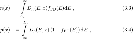
 atoms. The charge carrier densities at the point
  are expressed as
where
are expressed as
where  stands for the Fermi-Dirac distribution, which determines the occupation
of the conduction and valence band states and is given by Its validity rests upon thermal equilibrium between the charge carriers in a specific
region of the MOS device. This assumption is well justified when no voltage is
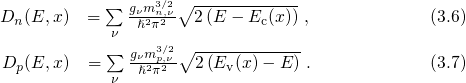
applied between source and drain of a MOSFET during NBTI stress. In the parabolic
band approximation the electron (
stands for the Fermi-Dirac distribution, which determines the occupation
of the conduction and valence band states and is given by Its validity rests upon thermal equilibrium between the charge carriers in a specific
region of the MOS device. This assumption is well justified when no voltage is
applied between source and drain of a MOSFET during NBTI stress. In the parabolic
band approximation the electron ( ) and hole (
 ) DOS in equation (3.3) and
(3.4) are defined by
) DOS in equation (3.3) and
(3.4) are defined by  is the electron/hole effective mass with a degeneracy of
  , where
  denotes the valley index.
  ,
,  , and
, and  stand for the Fermi energy, the
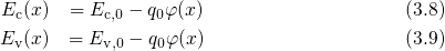
conduction, and the valence band edge, respectively. The electrostatic potential
stand for the Fermi energy, the
conduction, and the valence band edge, respectively. The electrostatic potential
 enters the calculation of the conduction (
 ) and the valence (
 )
band edge as follows:
)
band edge as follows:  and
and  denote the conduction and the valence band edge energy in the flat
band case, respectively. Due to the mutual dependence between
denote the conduction and the valence band edge energy in the flat
band case, respectively. Due to the mutual dependence between  , on the one
hand, and the carrier densities
, on the one
hand, and the carrier densities  and
and  , on the other hand, the equations
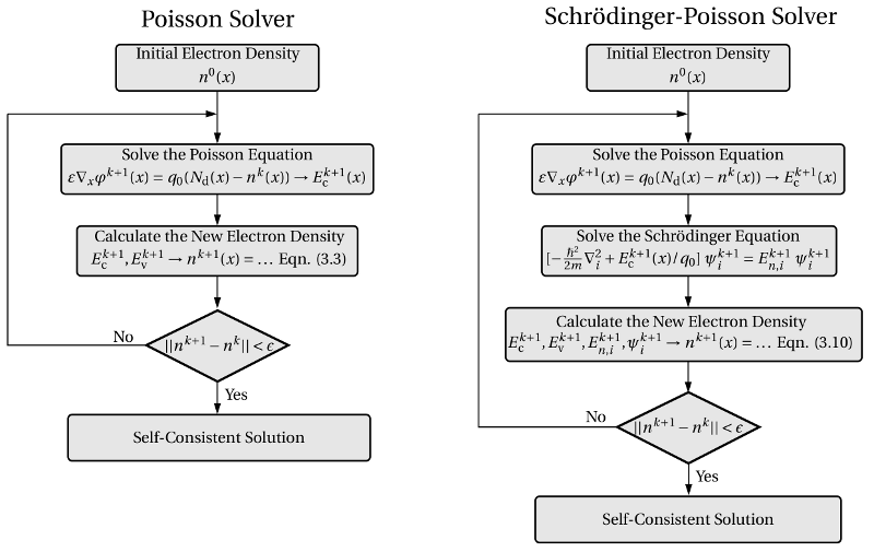
(3.1)-(3.9) must be solved self-consistently. This has been achieved by a P-solver,
whose functionality relies on a numerical iteration scheme, visualized in
Fig. 3.1.
, on the other hand, the equations
(3.1)-(3.9) must be solved self-consistently. This has been achieved by a P-solver,
whose functionality relies on a numerical iteration scheme, visualized in
Fig. 3.1.
More realistic simulations must account for the quantum confinement of the charge
carriers in the inversion layer. This effect arises from the band bending, which forms
a potential well for one type of charge carriers. As described in Section2.1, this
well enters as the potential in the one-dimensional Schrödinger equation,
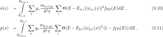
whose solution consists of the single quasi-bound states of electrons and
holes. These states are required for the calculation of the carrier densities
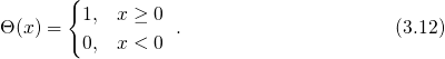
where  stands for the Heaviside step function defined by
  denotes the energy of the electron quasi-bound state
  and
and  is the
corresponding channel wavefunction. The single subbands of the quasi-bound states
add up to the electron DOS within the potential well, which is formed by
is the
corresponding channel wavefunction. The single subbands of the quasi-bound states
add up to the electron DOS within the potential well, which is formed by  and
limited by
and
limited by  . Outside this region, the charge carriers are calculated according
to equations (3.6) for the free states. Similarly, the hole quasi-bound states
. Outside this region, the charge carriers are calculated according
to equations (3.6) for the free states. Similarly, the hole quasi-bound states  with the channel wavefunction
  form subbands within the energy range between
 and
and  . For the calculation of the band diagram, the Poisson equation and
the Schrödinger equation must be solved self-consistently since they are
coupled through the electrostatic potential
. For the calculation of the band diagram, the Poisson equation and
the Schrödinger equation must be solved self-consistently since they are
coupled through the electrostatic potential  and the charge carrier
concentrations,
and the charge carrier
concentrations,  and
and  . In a SP-solver, this system of coupled
equations is treated using a self-consistent iteration method, outlined in Fig. 3.1.
Throughout this thesis, the Vienna Schrödinger Poisson (VSP) solver [130] has
been applied for the calculation of the band diagram and the charge carrier
concentrations.
. In a SP-solver, this system of coupled
equations is treated using a self-consistent iteration method, outlined in Fig. 3.1.
Throughout this thesis, the Vienna Schrödinger Poisson (VSP) solver [130] has
been applied for the calculation of the band diagram and the charge carrier
concentrations.


 enters the Poisson equation and a new
electrical potential
enters the Poisson equation and a new
electrical potential  is obtained, which is then required to calculate
the new electron density
is obtained, which is then required to calculate
the new electron density  . In a Poisson solver the new electron density
 is evaluated using the semi-classical formula (
 according to equation
(
according to equation
( , the iteration loop is continued at
the Poisson step until the update
, the iteration loop is continued at
the Poisson step until the update  falls below a certain limit
 .
.