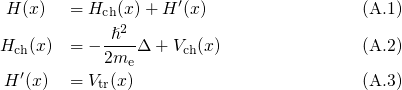
A.1 Fermi’s Golden Rule
Fermi’s golden rule provides one way to calculate the transition rate between two
certain quantum mechanically defined states. Due to its generality, it has various
applications in the field of atomic, nuclear, and solid-state physics. In the case of
NBTI, it is of most interest for charge transfer reactions and electron tunneling
in particular. In the following, Fermi’s golden rule is derived for electron
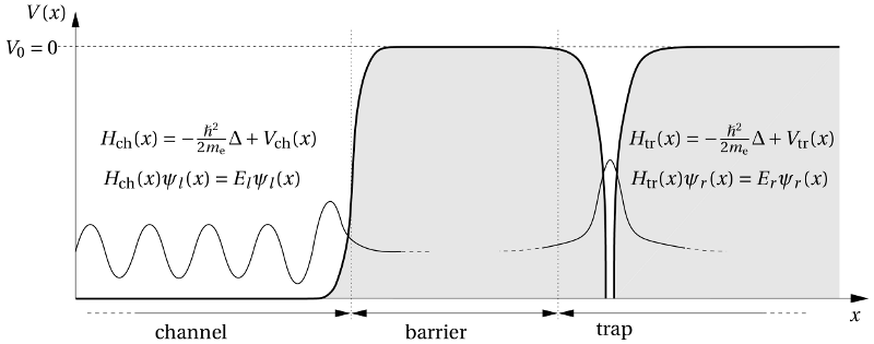
tunneling from the substrate into an oxide defect as illustrated in Fig. A.1.
The system is divided into three separate regions, namely the channel, the insulator
barrier, and the trap region. The electron wavefunctions  and
and  extend
into the classically forbidden barrier region. Their overlap actually leads to a
mutual influence between the channel and the trap system. However, this
influence is assumed to be negligible so that both systems can be treated
independently to first order. This justifies the assumption that in a first
approximation the channel and the trap system can be described by their own
Hamiltonians
extend
into the classically forbidden barrier region. Their overlap actually leads to a
mutual influence between the channel and the trap system. However, this
influence is assumed to be negligible so that both systems can be treated
independently to first order. This justifies the assumption that in a first
approximation the channel and the trap system can be described by their own
Hamiltonians  and
and  . For the derivation of the tunneling
rate, the Hamiltonian of the common system is taken as a starting point.
. For the derivation of the tunneling
rate, the Hamiltonian of the common system is taken as a starting point.
 is viewed as the time-dependent perturbation that triggers the scattering
from the band states
is viewed as the time-dependent perturbation that triggers the scattering
from the band states  into the trap states
  . The solution
  of the
common system
of the
common system  can be written as a linear combination of the eigen
wavefunctions
can be written as a linear combination of the eigen
wavefunctions  of the unperturbed system
  .
This expansion of the wavefunction is inserted into the time-dependent Schrödinger
equation and leads to Due to
.
This expansion of the wavefunction is inserted into the time-dependent Schrödinger
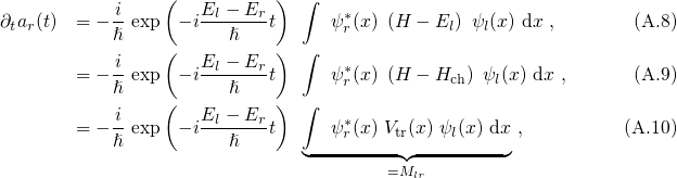
equation and leads to Due to 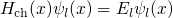 , the above equation simplifies to Multiplying both sides by
 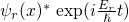 from the left and integrating over space
yields where
from the left and integrating over space
yields where  is referred to as the matrix element.
  gives the transition
probability
gives the transition
probability  that an electron initially located in the state
  , evolves into
the final states
, evolves into
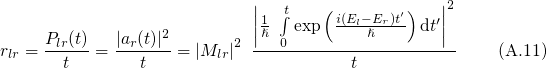
the final states  after a time t. Therefore, it must be divided by the time
  in
order to yield the transition rate
in
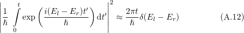
order to yield the transition rate  . The integrand is sharply peaked at
  and can be approximated as a
 -function. Substituting the integral in rate expression (A.11), one finally obtain ‘Fermi’s golden
rule’.
-function. Substituting the integral in rate expression (A.11), one finally obtain ‘Fermi’s golden
rule’.
 and
and  , respectively. This means that the attractive trap potential
 is not accounted for in
  so that
  in the trap
region. Vice versa, the channel potential
in the trap
region. Vice versa, the channel potential  is omitted in
  , which
consequently takes the value
, which
consequently takes the value  in the channel region.