2.3.4.2 Steady State

The trap occupation probability $f_t$ can be calculated by examining the steady state in which the following relation holds^2.12

$$R_n - G_n = R_p - G_p \ .$$ (2.211)

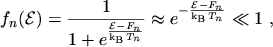
For the non degenerated case, that is, for the FERMI level several $\mathrm{k}_\mathrm{B}\, T_n$ below $\mathcal{E}_\mathrm{C}$, $\frac{\mathcal{E}- F_n}{\mathrm{k}_\mathrm{B}\, T_n} \gg 1$, MAXWELL-BOLTZMANN statistics can be assumed

$$f_n(\mathcal{E}) = \frac{1}{1 + e^\frac{\mathcal{E}- F_n}{\mathrm... ...}} \approx e^{- \frac{\mathcal{E}- F_n}{\mathrm{k}_\mathrm{B}\, T_n}} \ll 1 \ ,$$ (2.212)

which further allows to assume

$$(1 - f_n) \approx 1 \ .$$ (2.213)

Using the approximations (2.212) and (2.213) and the analog approximations for holes, equations (2.209) and (2.210) can be written as

$$R_n - G_n = \underbrace{c_n \, N_t}_{\textstyle 1 / \tau_n} \, \ensuremath{... ...m{B}\, T_\mathrm{L}}} \, f_t \Bigr) \,\, \ensuremath{\mathrm{d}}\mathcal{E}}\ ,$$ (2.214)

$$R_p - G_p = \underbrace{c_p \, N_t}_{\textstyle 1 / \tau_p} \, \ensuremath{... ... T_\mathrm{L}}} \, (1 - f_t) \Bigr) \,\, \ensuremath{\mathrm{d}}\mathcal{E}}\ ,$$ (2.215)

where $\tau_n$ and $\tau_p$ are the lifetimes for electrons and holes, respectively. The characteristic parameters describing the interaction of carriers and trap centers are the capture cross sections $\sigma_n$ and $\sigma_p$. If they are known the rate constants (and thus also the lifetimes) can be expressed as

$$c_n = \sigma_n \, v_{\mathrm{th},n} \ , \textcolor{lightgrey}{.......}c_p = \sigma_p \, v_{\mathrm{th},p} \ ,$$ (2.216)

where $v_{\mathrm{th},n}$ and $v_{\mathrm{th},p}$ are the thermal velocities of electrons and holes, respectively.

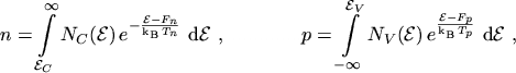
Using the following expressions for the electron and hole concentrations

$$n = \ensuremath{\int_{\mathcal{E}_C}^{\infty} N_C(\mathcal{E}) \,... ... F_p}{\mathrm{k}_\mathrm{B}\, T_p}} \,\, \ensuremath{\mathrm{d}}\mathcal{E}}\ ,$$ (2.217)

and the handy abbreviations $n_1$ and $p_1$ for the electron and hole concentrations when the FERMI level is equal to the trap level

$$n_1 = n(T_\mathrm{L}, F_n=\mathcal{E}_t) = \ensuremath{\int_{\mathcal... ...thrm{k}_\mathrm{B}\, T_\mathrm{L}}} \,\, \ensuremath{\mathrm{d}}\mathcal{E}}\ ,$$ (2.218)

$$p_1 = p(T_\mathrm{L}, F_p=\mathcal{E}_t) = \ensuremath{\int_{-\infty}... ...thrm{k}_\mathrm{B}\, T_\mathrm{L}}} \,\, \ensuremath{\mathrm{d}}\mathcal{E}}\ ,$$ (2.219)

eqns. (2.214) and (2.215) can be written as

$$R_n - G_n = \frac{1}{\tau_n} \, \Bigl( n \, (1 - f_t) - n_1 \, f_t \Bigr) \ ,$$ (2.220)

$$R_p - G_p = \frac{1}{\tau_p} \, \Bigl( p \, f_t - p_1 \, (1 - f_t) \Bigr) \ .$$ (2.221)

Making use of the steady state condition eqn. (2.211) the following expression for $f_t$ is found

$$f_t = \frac{n \, c_n + p_1 \, c_p}{c_n \, (n + n_1) + c_p \, (p +... ...rac{\tau_p \, n + \tau_n \, p_1}{\tau_p \, (n + n_1) + \tau_n \, (p + p_1)} \ .$$ (2.222)

Inserting eqn. (2.222) either in eqn. (2.214) or eqn. (2.215) yields the well known SHOCKLEY-READ-HALL net recombination rate

$$R = R_n - G_n = R_p - G_p = \frac{n \, p - n_i^2} {\tau_p \, (n +... ...+ \tau_n \, (p + p_1)} \ , \textcolor{lightgrey}{.......}n_1 \, p_1 = n_i^2 \ .$$ (2.223)

M. Gritsch: Numerical Modeling of Silicon-on-Insulator MOSFETs PDF