6.1 Temperature Tensor Modeling

To incorporate an anisotropic temperature into the standard energy transport model, it is of advantage to retain $T_n$ as the solution variable and to model $T_{xx}$ and $T_{yy}$ empirically by means of some anisotropy functions $\gamma_\nu(T_n)$

$$T_{xx} = \gamma_x \, T_n \ , \textcolor{lightgrey}{.......}T_{yy} = \gamma_y \, T_n \ .$$ (6.1)

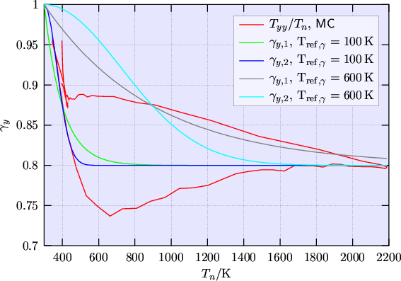
Fig. 6.1 shows the anisotropy function $\gamma_y$ obtained by Monte Carlo simulation. The two branches of the Monte Carlo results stem from the different circumstances in the regions of carrier heating and carrier cooling. Since modeling of the anisotropic temperature is only an approximation of a second-order effect, usage of a single valued function appears to be justified. An important property is that $\gamma_\nu(T_n)$ drops beginning from unity and saturates for high temperatures. This means that the distribution becomes anisotropic at high temperatures whereas the equilibrium distribution stays isotropic, which is consistent with the fact that the equilibrium solution of BOLTZMANN's transport equation is the isotropic MAXWELL distribution function.

Figure 6.1: Approximation of the anisotropic temperature by the analytical models.

Two analytical anisotropy functions shown in Fig. 6.1 have been investigated:

$$\gamma_{y, 1}(T_n) = \gamma_{0y} + \bigl( 1 - \gamma_{0y} \bigr) \, \exp \Bigl( - \frac{T_n - T_\mathrm{L}}{\mathrm{T_{ref, \gamma}}} \Bigr) \ ,$$ (6.2)

$$\gamma_{y, 2}(T_n) = \gamma_{0y} + \bigl( 1 - \gamma_{0y} \bigr) \, \exp \Bigl( - \Bigl( \frac{T_n - T_\mathrm{L}}{\mathrm{T_{ref, \gamma}}} \Bigr)^2 \Bigr) \ .$$ (6.3)

Implementation of both functions showed that the convergence properties are vastly improved by using eqn. (6.3) instead of eqn. (6.2). It is believed that the steep decrease of eqn. (6.2) near equilibrium and the non-vanishing derivatives under this conditions result in an unstable behavior. The analytical model for $T_{yy}$ using eqn. (6.3) is depicted in Fig. 6.2, with $\gamma _{0y}=0.75$ and $\mathrm{T_{ref, \gamma}} = 600 \, \mathrm{K}$. Excellent agreement with the Monte Carlo data is obtained.

Figure 6.2: Components of the temperature tensor obtained by Monte Carlo simulations compared to the analytical model of $T_{yy}$.

M. Gritsch: Numerical Modeling of Silicon-on-Insulator MOSFETs PDF