The finite volume method is the most natural discretization scheme, because it makes use of the conservation laws in integral form. It subdivides the domain into cells and evaluates the field equations in integral form on these cells. In the area of TCAD this method is often called the finite box method [26] to express the geometrical origin of the discretized domain. Most applications of the finite volume method do not include the time variable, which has to be enforced by a separate discretization. The concepts and implementation are simple for different dimensions and different types of cell complexes.
For the finite volume method the domain
![]() is first subdivided
into non-overlapping control volumes
is first subdivided
into non-overlapping control volumes ![]() of a cell complex
of a cell complex
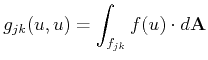
![]() . In each control volume an integral conservation law
is imposed [27]:
. In each control volume an integral conservation law
is imposed [27]:
 |
(2.10) |
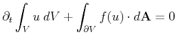
By the step towards the discrete space, the integral conservation law is transfered to small control volumes:
 |
(2.11) |
The integral conservation law is readily obtained upon spatial
integration of, e.g., a divergence equation in a region
![]() . The choice of control volume tessellation is flexible in
the finite volume method. The primary requirement is a secondary mesh
(see Figure 2.4) with special
properties related to the primary mesh.
. The choice of control volume tessellation is flexible in
the finite volume method. The primary requirement is a secondary mesh
(see Figure 2.4) with special
properties related to the primary mesh.
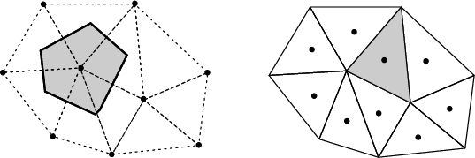 |
In a vertex-centered method the control volumes are formed as a geometric dual to the cell complex and unknown solutions are stored on a per-vertex basis. In the cell-centered method the cells serve directly as control volumes containing the unknown solutions (degrees of freedom) stored on a per-cell basis. See Figure 2.5 for a graphical depiction of these two methods. The integral conservation law is enforced for each control volume and for the entire domain. To obtain a linear system of algebraic equations, integrals must be expressed in terms of mean values.
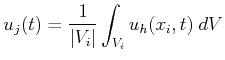
Two assumptions are fundamental to the finite volume method. First, a piecewise constant cell average is introduced for each control volume:
![\begin{figure}\begin{center}
\small\psfrag{f} [c]{$\mathrm{u}$}\psfrag{x} [c...
...e=figures/fv_ansatz_function.eps, width=0.4\textwidth}\end{center}\end{figure}](img473.png) |
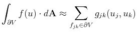
Second, the true flux at the interfaces is replaced by a
numerical flux function
![]() . For arbitrary spatial dimensions, the flux
integral is approximated by a numerical integration scheme, e.g., by a
quadrature rule:
. For arbitrary spatial dimensions, the flux
integral is approximated by a numerical integration scheme, e.g., by a
quadrature rule:
The numerical flux has to satisfy the following properties:
| (2.14) |
 |
(2.15) |
Using Equation 2.12 and the previous interpretation of finite volumes for stationary meshes produces the following evolution equation for cell averages:
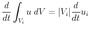 |
(2.16) |
One of the simplest finite volume schemes in a semi-discrete
formulation can be obtained by utilizing representations which are
continous in time,
![]() , and piecewise constant in
space,
, and piecewise constant in
space,
![]() such that:
such that:
 |
(2.17) |
with initial data
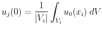 |
(2.18) |
and the numerical flux functions
![]() given by the
following system of ordinary differential equations:
given by the
following system of ordinary differential equations:
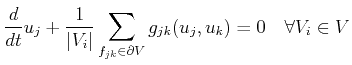 |
(2.19) |
The final remaining issue is that the solution is available only at the computational nodes, the control volume centers. Interpolation is needed to obtain the function values at the vertices.
Using an explicit or implicit time integration formula [67], e.g., a forward Euler scheme:
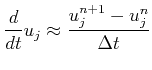 |
(2.20) |
produces a fully-discrete finite volume form:
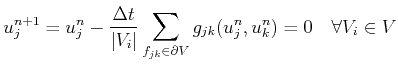 |
(2.21) |