7.4 Multivariate Bernstein Polynomials

In order to keep the formulae simple we will again only consider functions defined on the multidimensional intervals $[0,1]\times\cdots\times[0,1]$, i.e., the unit cube in  $\mathbb{R}^N$. Using affine transformations it is straightforward to apply the formulae and results to arbitrary intervals. The proofs from this section can be found in Appendix B.

To illustrate the general concept we first look at the two-dimensional case. We obtain the desired approximation by first approximating one variable and then the second.

Theorem 7..6   Let $f: I:=[0,1]\times[0,1]\to\mathbb{R}$ be a continuous function. Then the two-dimensional Bernstein polynomials

$$B_{f,n_1,n_2}(x_1,x_2):=\sum_{k_1=0}^{n_1}\sum_{k_2=0}^{n_2} f \l... ... k_1} {n_2\choose k_2} x_1^{k_1} (1-x_1)^{n_1-k_1} x_2^{k_2} (1-x_2)^{n_2-k_2}$$

converge pointwise to $f$ for $n_1,n_2\to\infty$.

We define now the multivariate Bernstein polynomials as follows.

Definition 7..7 (Multivariate Bernstein Polynomials)   Let $n_1,\ldots,n_m\in\mathbb{N}$ and $f$ be a function of $m$ variables. The polynomials

$$B_{f,n_1,\ldots,n_m}(x_1,\ldots,x_m):= \sum_{{0\le k_j\le n_j}\at... ...ght) \prod_{j=1}^m \left( {n_j\choose k_j} x_j^{k_j} (1-x_j)^{n_j-k_j} \right)$$

are called the multivariate Bernstein polynomials of $f$.

We note that $B_{f,n_1,\ldots,n_m}$ is a linear operator.

Theorem 7..8 (Pointwise Convergence)   Let $f: [0,1]^m\to\mathbb{R}$ be a continuous function. Then the multivariate Bernstein polynomials $B_{f,n_1,\ldots,n_m}$ converge pointwise to $f$ for $n_1,\ldots,n_m\to\infty$.

But using this straightforward method we can only prove pointwise convergence.

Lemma 7..9   For all $x\in\mathbb{R}$

$$\sum_{k=0}^{n} (k-nx)^2 {n\choose k} x^k (1-x)^{n-k} = nx(1-x).$$

For all $x\in[0,1]$ we have $x(1-x)\le 1/4$ and hence

$$0 \le \sum_{k=0}^{n} (k-nx)^2 {n\choose k} x^k (1-x)^{n-k} \le {n\over 4}.$$

Theorem 7..10 (Uniform Convergence)   Let $f: [0,1]^m\to\mathbb{R}$ be a continuous function. Then the multivariate Bernstein polynomials $B_{f,n_1,\ldots,n_m}$ converge uniformly to $f$ for $n_1,\ldots,n_m\to\infty$.

A reformulation of this fact is the following corollary. It ensures that all functions considered in TCAD applications can be approximated arbitrarily well.

Corollary 7..11   The set of all polynomials is dense in $C([0,1]^m)$.

By presupposing more knowledge about the rate of change of the function, namely a Lipschitz condition, an error bound is obtained.

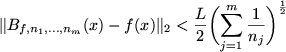
Theorem 7..12 (Error Bound for Lipschitz Condition)   If $f: I:=[0,1]^m\to\mathbb{R}$ is a continuous function satisfying the Lipschitz condition

$$\Vert f(x)-f(y)\Vert _2 < L \Vert x-y\Vert _2$$

on $I$, then the inequality

$$\Vert B_{f,n_1,\ldots,n_m}(x) - f(x) \Vert _2 < {L\over2} \biggl( \sum_{j=1}^m {1\over n_j} \biggr)^{1\over2} %$$

holds.

The following asymptotic formula gives us information about the rate of convergence.

Theorem 7..13 (Asymptotic Formula)   Let $f: I:=[0,1]^m\to\mathbb{R}$ be a $C^2$ function and $x\in I$, then

$$\lim_{n\to\infty} n ( B_{f,n,\ldots,n}(x) - f(x) ) = \sum_{j=1}^m... ...rtial x_j^2} \le {1\over8} \sum_{j=1}^m {\partial ^2 f(x)\over\partial x_j^2}.$$

The asymptotic formula states that the rate of convergence depends only on the partial derivatives $\partial ^2 f(x)/\partial x_j^2$. This is noteworthy, since it is often the case that the smoother a function is and the more is known about its higher derivatives, the more properties can be proven, but in this case only the second order derivatives play a role.