Next: 4. Monte Carlo Technique
Up: Dissertation Gerhard Karlowatz
Previous: 2. Strained Band Structure
Subsections
3. The Semiclassical Transport Model
As computational power raises and more efficient new Monte Carlo algorithms are
developed, the Monte Carlo approach to solve the Boltzmann equation for TCAD
device simulation is getting more and more important. In this work the
Boltzmann equation - originally developed to describe the flow of kinetic
gases - is used with extensions to meet the properties of quantum mechanical
transport occurring for electron or hole ensembles in crystals. These
extensions include particle kinetics depending on a position-dependent band
structure and on scattering events, which are calculated quantum-mechanically
using Fermi's Golden Rule. The carrier motion consists of periods of
collisionless acceleration caused by external forces, interrupted by
instantaneous scattering events. The Monte Carlo approach solves the
semiclassical Boltzmann transport equation [Kosina00].
During this work our in-house Monte Carlo tool named VMC [IuE06] was further developed in general and
extended by a FBMC part. This chapter gives an overview of the used Monte Carlo models
and algorithms with focus on the numerical methods used for CPU time efficient FBMC simulation.
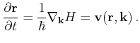
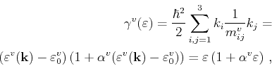
3.1 The Equations of Motion
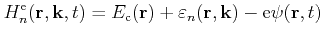
The semiclassical Hamilton function
 for an electron in a conduction band is given by
 |
(3.1) |
where  is the conduction band edge,
 is the energy of the
  -th band
relative to the conduction band edge,
-th band
relative to the conduction band edge,  is the electrostatic potential,
 is the position,
 is the wave vector of the
carrier, and e the elementary charge. The Hamilton function for holes reads
is the wave vector of the
carrier, and e the elementary charge. The Hamilton function for holes reads
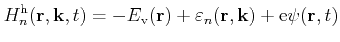 |
(3.2) |
where
 is the valence band edge.
The collisionless motion of the carriers is described by the equations of
motions given by Newton's law
is the valence band edge.
The collisionless motion of the carriers is described by the equations of
motions given by Newton's law
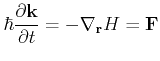 |
(3.3) |
and the carrier group velocity
 |
(3.4) |
Here,  is the reduced Planck constant,
 denotes the force and
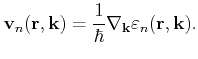
 the group velocity. In the semiclassical Monte Carlo framework the
velocity
the group velocity. In the semiclassical Monte Carlo framework the
velocity
 for a carrier in the band
is the group velocity of the
wave packet of the carrier and follows from (3.4)
for a carrier in the band
is the group velocity of the
wave packet of the carrier and follows from (3.4)
 |
(3.5) |
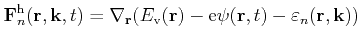
The force
denotes
 |
(3.6) |
for electrons and
 |
(3.7) |
for holes.
3.2 The Boltzmann Transport Equation
Because of the nature of scattering as a random process it is
impossible to determine the path of a carrier exactly. Instead a stochastic approach
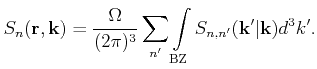
is used where the carrier gas is described by a distribution function
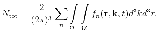
 . This distribution function is related to the total
number of particles
. This distribution function is related to the total
number of particles
 in the system by
 |
(3.8) |
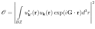
The integral in real space is hereby over the whole device domain  whereas
the integral in
-space is over the first Brillouin zone (BZ),
whereas
the integral in
-space is over the first Brillouin zone (BZ),
 is the minimum phase-space volume of a particle and the
factor of two originates from the two possible spin states of the carriers.
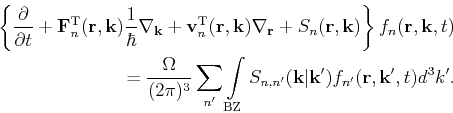
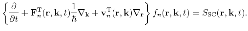
The semiclassical Boltzmann equation reads then
is the minimum phase-space volume of a particle and the
factor of two originates from the two possible spin states of the carriers.
The semiclassical Boltzmann equation reads then
 |
(3.9) |
The left hand side is derived from the equations of motion (3.2) and (3.3).
 is the
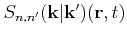
scattering integral given by
is the
scattering integral given by
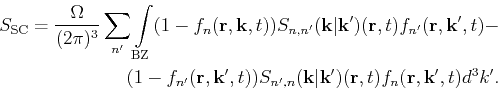 |
(3.10) |
describes the transition from a state
 into a state
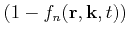
 and the inverse process. The rate for a
transition from an initial state
to a final state
is proportional to the probabilities that the initial
state is occupied,
and the inverse process. The rate for a
transition from an initial state
to a final state
is proportional to the probabilities that the initial
state is occupied,
 , and that the final state is
not occupied,
, and that the final state is
not occupied,
 , and to the transition rate
 . The factor
stems from the Pauli exclusion principle.
. The factor
stems from the Pauli exclusion principle.
The Boltzmann equation in the form of (3.9) is non-linear, because the
transition rate may depend on the carrier distribution and the scattering
integral includes a product of the distribution function with itself. The
latter can be avoided if the Pauli exclusion principle is neglected. If
additionally it is assumed, that the transition rate does not depend on
the distribution function, we achieve the linear Boltzmann
equation
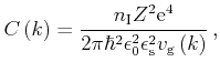
The scattering rate
 is the rate at which
carriers are scattered out of their initial state and is defined as
is the rate at which
carriers are scattered out of their initial state and is defined as
 |
(3.12) |
Equation (3.11) describes the kinetics of a carrier ensemble where the
particles are considered independent and noninteracting.
3.3 Scattering Mechanisms
In this work scattering is treated on the basis of Fermi's Golden Rule [Landau81]
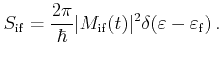 |
(3.13) |
Here,
 is the transition probability from the initial state i to the
final state f and
is the transition probability from the initial state i to the
final state f and
 is the energy of the final state. The matrix
element
is the energy of the final state. The matrix
element
 is given by
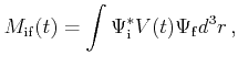 |
(3.14) |
where
 and
and
 are the wave functions of the
initial and final state, respectively.
are the wave functions of the
initial and final state, respectively.  is the perturbation potential.
The density of states per spin of a band
is given by
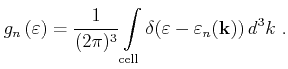 |
(3.15) |
The density of states integral can be evaluated numerically as for FBMC
simulation or approximated by analytical expressions. Following the approach of
Jacoboni [Jacoboni83] an analytical description for the conduction bands
is derived by approximating the minima of the conduction bands - the so called
valleys - by using the bandform function
 |
(3.16) |
where  denotes the valley index and
 is the energy relative to the
valley energy offset
is the energy relative to the
valley energy offset
 . One can include strain effects by introducing
for each valley strain-dependent effective mass tensors
. One can include strain effects by introducing
for each valley strain-dependent effective mass tensors
 , nonparabolicity
coefficients
, nonparabolicity
coefficients
 , and valley energy offsets. If
  is set to
zero the shape of the band approximation simplifies from nonparabolic to
parabolic. The density of states of a nonparabolic band can be
written as
is set to
zero the shape of the band approximation simplifies from nonparabolic to
parabolic. The density of states of a nonparabolic band can be
written as
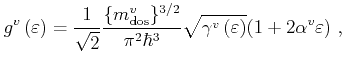 |
(3.17) |
where
 is the density of states effective mass of the
-th valley,
which can be obtained from the effective mass tensor
is the density of states effective mass of the
-th valley,
which can be obtained from the effective mass tensor
![$\displaystyle m^v_\mathrm{dos}= \sqrt[3]{ m_{11}^v m_{22}^v m_{33}^v } .%\vphantom{\sum_i}
$](img268.png) |
(3.18) |
The approach to use valley-dependent scattering models
can be adapted from Monte Carlo with analytical band structure models to fit
into the framework of FBMC [Jungemann03]. The first Brillouin
zone of the first conduction band of Si is divided into six volumes  as
defined in Table 3.1 where
indices the
-th valley in the
-th
band.
The same approximation is also applied to the higher conduction bands. This
approach is in the spirit of the analytical many valley model
[Jacoboni83]. In combination with constant matrix elements it gives a CPU
efficient formulation of the scattering rates,
because scattering rates are proportional to the density of
states, which is calculated numerically from the full-band structure.
as
defined in Table 3.1 where
indices the
-th valley in the
-th
band.
The same approximation is also applied to the higher conduction bands. This
approach is in the spirit of the analytical many valley model
[Jacoboni83]. In combination with constant matrix elements it gives a CPU
efficient formulation of the scattering rates,
because scattering rates are proportional to the density of
states, which is calculated numerically from the full-band structure.
Table 3.1:
The six volumes in the first Brillouin representing the six X-valleys of the first conduction band.
|
|
3.3.1 Phonon Scattering
The transition rate from an initial state (
 ) to a final state
(
) to a final state
(
 ) for phonon scattering in a non-polar semiconductor can be
written as [Jacoboni83]
) for phonon scattering in a non-polar semiconductor can be
written as [Jacoboni83]
![$\displaystyle \{\tiny S^{ \shortstack{abs [-2pt] emi }} \} ^{v'v}(\mathbf{k}...
...repsilon ^{v'}(\mathbf{k}') - \varepsilon ^{v}(\mathbf{k}) \mp \hbar\omega_q] $](img291.png) |
(3.19) |
Here, the upper and lower signs denote phonon absorption and emission,
respectively. The rate depends on the the phonon number  , the momentum transfer
 , the deformation potential tensor
 , the mass density of the crystal
  , the overlap integral
 , the phonon angular
frequency
, the phonon angular
frequency  and its polarization
  .
.
The overlap integral
 |
(3.20) |
depends on the type of transition. For intravalley transitions of electrons it
is common to set
to unity, which is exact only for wave functions
of pure  -states or for exact plane waves [Jacoboni83]. The
lowest conduction band of cubic semiconductors is a mixture of a
and
-states or for exact plane waves [Jacoboni83]. The
lowest conduction band of cubic semiconductors is a mixture of a
and
 -type states and so overlap factors less than unity are obtained.
Since for both intra- and intervalley transitions the overlap factors
were found to
be almost constant [Reggiani73] the values for
can be
included in the coupling constants.
-type states and so overlap factors less than unity are obtained.
Since for both intra- and intervalley transitions the overlap factors
were found to
be almost constant [Reggiani73] the values for
can be
included in the coupling constants.
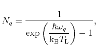
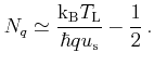
The phonon number
is given by the Bose-Einstein statistics
 |
(3.21) |
where
 denotes the lattice temperature and
 the Boltzmann constant.
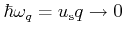
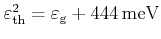
Since at room temperature the acoustic phonon energy
the Boltzmann constant.
Since at room temperature the acoustic phonon energy
 is very small compared to
the thermal energy
is very small compared to
the thermal energy
 the expression for the transition rate
for acoustic intravalley scattering can be simplified by using the elastic and
equipartition approximation. Within the latter approximation the Bose-Einstein
statistics (3.21) is replaced by its first order Taylor expansion which gives for the
phonon population
the expression for the transition rate
for acoustic intravalley scattering can be simplified by using the elastic and
equipartition approximation. Within the latter approximation the Bose-Einstein
statistics (3.21) is replaced by its first order Taylor expansion which gives for the
phonon population
 |
(3.22) |
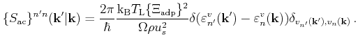
The phonon dispersion relation for small
 is approximated as
 . Thus, (3.19) becomes
![$\displaystyle \{ S_\mathrm{ac}^{\tiny\shortstack{abs [-2pt] emi }} \} ^{v}(\...
...[\varepsilon ^{v}(\vect{k}') - \varepsilon ^{v}(\vect{k})\pm \hbar \omega_q] ,$](img309.png) |
(3.23) |
where
 denotes the average sound velocity and
is the mass density of the crystal.
denotes the average sound velocity and
is the mass density of the crystal.
 is the acoustic
deformation potential of the
-th valley, which is derived by averaging the
two non-zero elements of the deformation potential tensor over the polar
angle [Jacoboni83].
is the acoustic
deformation potential of the
-th valley, which is derived by averaging the
two non-zero elements of the deformation potential tensor over the polar
angle [Jacoboni83].
In the elastic approximation the phonon energy is neglected,
 . Therefore, emission and absorption processes
are equivalent and the transition probabilities can be added.
This leads to a scattering rate for acoustic intraband scattering which
is a function of energy only
. Therefore, emission and absorption processes
are equivalent and the transition probabilities can be added.
This leads to a scattering rate for acoustic intraband scattering which
is a function of energy only
 |
(3.24) |
In (3.24),
 denotes the density of
states of valley
. The values of the parameters used in
(3.24) can be found in
Table
denotes the density of
states of valley
. The values of the parameters used in
(3.24) can be found in
Table ![[*]](crossref.png) .
.
Table 3.2:
Parameters for acoustic and optical intravalley phonon scattering in Si.
|
|
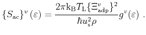
When the lattice temperature is very low (3.22) does not hold anymore
and the dependence on the acoustic phonon energy and momentum transfer have to be
considered. Using a model in which the phonon dispersion
has to be evaluated during simulation will demand long calculation
times. Therefore it is useful to derive a temperature-dependent but otherwise
constant mean phonon energy
 and formulate the
acoustic intraband scattering rate as [R.-Bolívar05]
[Bufler01]
and formulate the
acoustic intraband scattering rate as [R.-Bolívar05]
[Bufler01]
![$\displaystyle \{ S_\mathrm{ac}^{\tiny\shortstack{abs [-2pt] emi }} \} ^v\lef...
...} \mp \frac{1}{2} \right ) g^{v}(\varepsilon \pm \hbar \omega_{\mathrm{ac}}) .$](img330.png) |
(3.25) |
To obtain the average momentum transfer
 a
mean momentum transfer
a
mean momentum transfer
 is calculated first by taking an
average over the solid angle
is calculated first by taking an
average over the solid angle
 |
(3.26) |
This result is used to take a second average with the equilibrium distribution
function, i.e., the Maxwell-Boltzmann distribution
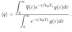 |
(3.27) |
With a parabolic band approximation
evaluates to
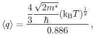 |
(3.28) |
where  is the effective electron mass.
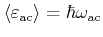
Now, the average phonon energy is obtained by assuming a linear dispersion relation
is the effective electron mass.
Now, the average phonon energy is obtained by assuming a linear dispersion relation
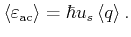 |
(3.29) |
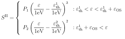
From the matrix element theorem one can derive that optical intravalley
scattering occurs only in the conduction band valleys along the
 directions [Harrison56]. Thus this type of scattering is
important in Ge. In Si it contributes only at high electron energies.
directions [Harrison56]. Thus this type of scattering is
important in Ge. In Si it contributes only at high electron energies.
By replacing
 in (3.19) with a squared optical
coupling constant the scattering probability can be reformulated with a squared
optical coupling constant
in (3.19) with a squared optical
coupling constant the scattering probability can be reformulated with a squared
optical coupling constant
 [Jacoboni83].
The optical phonon energies
[Jacoboni83].
The optical phonon energies
 and the phonon number
 can be assumed to be constant since the dispersion curve is nearly flat for
phonons involved in optical intraband transitions. If the overlap factor
is lumped in the coupling constant the resulting transition rate
can be written as
can be assumed to be constant since the dispersion curve is nearly flat for
phonons involved in optical intraband transitions. If the overlap factor
is lumped in the coupling constant the resulting transition rate
can be written as
![$\displaystyle \{ S_\mathrm{op}^{\tiny\shortstack{abs [-2pt] emi }} \} ^{v}(\...
...on ^{v}(\vect{k}') - \varepsilon ^v(\vect{k}) \mp \hbar\omega_{\mathrm{op}}] .$](img342.png) |
(3.30) |
With the above formulation the scattering rate for optical phonons is a
function of the final energy

![$\displaystyle \{ S_\mathrm{op}^{\tiny\shortstack{abs [-2pt] emi }} \} ^v\lef...
...{1}{2} \right ) g^{v}\left(\varepsilon \pm \hbar \omega_{\mathrm{op}}\right) .$](img344.png) |
(3.31) |
The values used for optical intravalley scattering are given in Table .
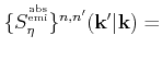
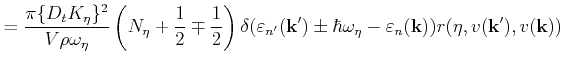
Intervalley Phonon Scattering
Both acoustic and optical phonons can cause electron transitions between
states in different conduction band valleys [Harrison56,Conwell67].
The scattering rate for intervalley scattering out of a valley
for a phonon
mode  reads
reads
![$\displaystyle \{ S_\eta^{\tiny\shortstack{abs [-2pt] emi }} \} ^{v}\left(\va...
...(\varepsilon ^{v'} \pm \hbar \omega_\eta - \Delta \varepsilon ^{v'v}\right) .$](img346.png) |
(3.32) |
The possible final valleys  are determined by two selection rules for the
phonon mode
:
are determined by two selection rules for the
phonon mode
:  -type phonons induce transitions between opposite valleys
on the same axis in
-type phonons induce transitions between opposite valleys
on the same axis in
 space, and
  -type phonons induce transitions among orthogonal
axes. The coupling constants
-type phonons induce transitions among orthogonal
axes. The coupling constants
 depend on the phonon branch
and the initial and final valley in a particular transition.
depend on the phonon branch
and the initial and final valley in a particular transition.  denotes the number of possible final equivalent valleys in a transition,
 is the phonon number, and
 is the energy difference
between the minima of the final and initial valley.
is the energy difference
between the minima of the final and initial valley.
The numerical values for the bulk phonon scattering rates are
summarized in Table 3.3.
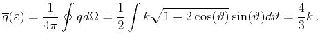
Figure 3.1 depicts the low field electron mobility over temperature. This
result is obtained by Monte Carlo simulation including only phonon scattering
and agrees very well with simulation data from [Canali75]. Because of the
influence of impurity scattering the mobility obtained from experimental data
is lower in the low temperature regime.
Figure 3.1:
Low field electron mobility in Si versus lattice
temperature as a result of Monte Carlo simulation (VMC) compared to experimental and
theoretical data [Canali75].
|
|
Table 3.3:
Phonon modes, coupling constants, phonon energies, and selection rule for Si as used
in the analytical intervalley phonon scattering model. Values are taken
from [Jacoboni83].
| Phonon Mode
|


|


|
Selection Rule 
|
| Transversal acoustic |
50 |
12.06 |
g |
| Longitudinal acoustic |
80 |
18.53 |
g |
| Longitudinal optical |
1100 |
62.04 |
g |
| Transversal acoustic |
30 |
18.86 |
f |
| Longitudinal acoustic |
200 |
47.39 |
f |
| Transversal optical |
200 |
59.03 |
f |
|
As explained in the introduction of Section 3.3, the many-valley approach
for analytical band models is adapted for the full-band framework. The differences
in the formulation of the scattering rates lie then in the analytical versus
the numerical calculation of the density of states and the implementation of
interband transitions.
Table 3.4:
Phonon modes, coupling constants, phonon energies, and phonon branch of inelastic phonon scattering for Si [Dhar06] as used in FBMC simulation.
| Phonon Mode
|
|
|
Selection Rule
|
| Transversal acoustic |
47.2 |
12.1 |
g |
| Longitudinal acoustic |
75.5 |
18.5 |
g |
| Longitudinal optical |
1042 |
62.0 |
g |
| Transversal acoustic |
34.8 |
19.0 |
f |
| Longitudinal acoustic |
232 |
47.4 |
f |
| Transversal optical |
232 |
58.6 |
f |
| Holes acoustic |
991 |
63.3 |
a |
|
Table 3.5:
Phonon modes, coupling constants, phonon energies, and phonon branch of inelastic phonon scattering for Ge [Jungemann03] as used in FBMC simulation.
| Phonon Mode
|
|
|
Selection Rule
|
| Transversal acoustic |
47.9 |
5.6 |
g |
| Longitudinal acoustic |
77.2 |
8.6 |
g |
| Longitudinal optical |
928 |
37.0 |
g |
| Transversal acoustic |
283 |
9.9 |
f |
| Longitudinal acoustic |
1940 |
28.0 |
f |
| Transversal optical |
1690 |
32.5 |
f |
| Holes acoustic |
3500 |
37.0 |
a |
|
The transition rate of full-band acoustic intravalley scattering is derived by
applying the elastic approximation to (3.23)
 |
(3.33) |
The deformation potentials  are assumed to be 8.5 eV for electrons and
5.12 eV [Dhar06] for holes in Si [Dhar06] and 8.79 eV for electrons
and 7.40 eV for holes in Ge [Jungemann03]. The Kronecker delta term on the right
hand side defines that transitions are allowed only within a valley
, but
between different bands
are assumed to be 8.5 eV for electrons and
5.12 eV [Dhar06] for holes in Si [Dhar06] and 8.79 eV for electrons
and 7.40 eV for holes in Ge [Jungemann03]. The Kronecker delta term on the right
hand side defines that transitions are allowed only within a valley
, but
between different bands  and
. The probability to scatter to another
band
is determined by the contribution of the density of states in this
band at the final energy.
and
. The probability to scatter to another
band
is determined by the contribution of the density of states in this
band at the final energy.
For the simulation of SiGe alloys the parameter values for Si
and Ge are linearly interpolated according to the material composition. Since
only the  -valleys are considered in the the implemented full-band
scattering formalism, simulation of SiGe compounds is only valid as long as the
-valleys are dominantly populated.
-valleys are considered in the the implemented full-band
scattering formalism, simulation of SiGe compounds is only valid as long as the
-valleys are dominantly populated.
The coupling constants, phonon energies, and phonon modes
, and the
selection rule
for inelastic full-band phonon scattering in Si are shown in
Table 3.4. The coupling constants are taken from
[Jacoboni83] and [Jungemann03] and are fine-tuned to match the measured
data for biaxial strained Si [Dhar06]. Table 3.5 shows the
respective values for Ge, which are used to calculate the interpolated
parameter values of SiGe alloys.
The phonon branches determine
a set of selection rules labeled
 . In
the full-band formulation these selection rules act on the density of states
whereas the coupling constant is kept constant for all combination of valleys
and bands. This leads to the expression
. In
the full-band formulation these selection rules act on the density of states
whereas the coupling constant is kept constant for all combination of valleys
and bands. This leads to the expression
 |
(3.34) |
for the transition rate due to intervalley phonon scattering. For holes there is no
restriction in the selection of the final state by a selection rule and
there is only one inelastic optical phonon mode.
Figure 3.2 shows the electron velocity for relaxed Si as a function of the
electric field in  direction. It can be observed that the
data from VMC agrees well with measurements.
direction. It can be observed that the
data from VMC agrees well with measurements.
Figure 3.3 depicts the
hole velocity as a function of the electric field and
Figure 3.4 the energy as a function of the electric field in
direction for relaxed Ge. These results are compared to values
from literature [Fischetti96a][Yamada95][Ghosh06] and show good agreement.
Figure 3.2:
Electron velocity versus field in [100]
direction for relaxed Si. Monte Carlo results (VMC) are compared to
measurement [Canali75].
Figure 3.3:
Hole velocity versus field in
[100] direction for relaxed Ge. Monte Carlo results (VMC) are compared to
results from literature [Fischetti96a][Yamada95][Ghosh06].
|
|
Figure 3.4:
Hole energy versus field in
[100] direction for relaxed Ge. Monte Carlo results (VMC) are compared to
results from literature [Fischetti96a][Yamada95][Ghosh06].
|
|
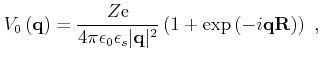
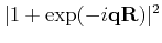
In this work the well known model of Brooks and Herring [Brooks51] is used
in an extended form, where multi-potential scattering and dispersive screening
is included. The Fourier transformed potential
 of a screened,
ionized impurity is given by
of a screened,
ionized impurity is given by
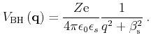 |
(3.35) |
Here,
 is the charge of the impurity center
and
is the charge of the impurity center
and
 is the inverse Thomas-Fermi screening length
 |
(3.36) |
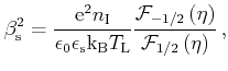
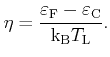
where
 is the concentration of the impurity centers and
 denotes the Fermi integral of the
  -th order with the
reduced Fermi energy
as argument
-th order with the
reduced Fermi energy
as argument
 |
(3.37) |
Application of the Golden Rule (3.13) and the scattering potential (3.35) gives the transition rate
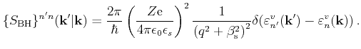 |
(3.38) |
The ionized impurity scattering rate from the above potential can be
formulated [Kosina98]
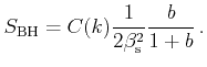 |
(3.39) |
Here,
 and the prefactor
 is set
 |
(3.40) |
where
 denotes the magnitude of the group velocity. In the
approximation based on non-parabolic analytic bands, the scattering rate
for a valley
evaluates to
denotes the magnitude of the group velocity. In the
approximation based on non-parabolic analytic bands, the scattering rate
for a valley
evaluates to
 |
(3.41) |
with
 |
(3.42) |
The Brooks-Herring model significantly overestimates the mobility
for higher impurity concentrations. To extend the validity of the model,
multi-potential scattering and dispersive screening via Lindhard's dielectric
function is included.
Multi potential scattering to the first order considers only the Coulomb interaction
of the carrier with pairs of impurities. The Fourier transform of the applied
potential takes the form:
 |
(3.43) |
where
 is the distance between the centers.
 is the total potential which forms because of the response of
the electrons to the applied potential
is the total potential which forms because of the response of
the electrons to the applied potential
 . The total potential is
related to the applied potential via the dielectric function
. The total potential is
related to the applied potential via the dielectric function

 |
(3.44) |
The frequency  equals zero because the applied potential is time
independent.
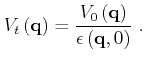
When considering only low order screening effects, Lindhard's dielectric
function is appropriate [Ferry91]:
equals zero because the applied potential is time
independent.
When considering only low order screening effects, Lindhard's dielectric
function is appropriate [Ferry91]:
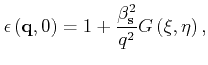 |
(3.45) |
Here,
 denotes the screening function for which an
integral representation exists [Ferry91]
denotes the screening function for which an
integral representation exists [Ferry91]
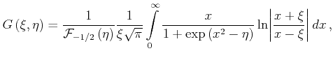 |
(3.46) |
with
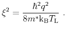 |
(3.47) |
The integral (3.46) cannot be evaluated analytically, but there are
attempts in literature to approximate it with a sufficiently accurate rational
expression [Kosina98]. After combining equations (3.43)(3.44)
and (3.45) and averaging the term
 over the solid
angle
over the solid
angle
 is found as
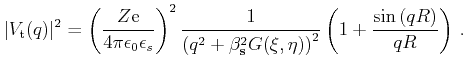 |
(3.48) |
Figure 3.5:
Electron low field mobility versus doping concentration for Si. Experimental data [Masetti83] are compared to Monte Carlo results. An ionized impurity model which includes a two-ion potential and
dispersive screening is used for the Monte Carlo simulation.
|
|
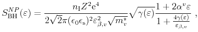
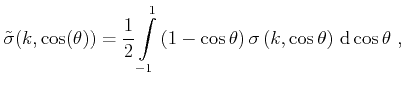
The long range of the Coulomb force causes a large scattering cross section of
a single ion. This makes Coulomb scattering occur very frequently and consume a
high amount of computation time during a Monte Carlo simulation.
The momentum transfer per scattering event is rather small.
This leads to a very anisotropic scattering behavior with a high percentage of small-angle scattering events.
The number of scattering events can be significantly reduced by the
introduction of an isotropic equivalent scattering cross section
 ,
which has the same momentum relaxation time as
the original cross section
,
which has the same momentum relaxation time as
the original cross section  . These cross sections are
related by [Kosina97]
. These cross sections are
related by [Kosina97]
 |
(3.49) |
where  is the angle between
and
is the angle between
and
 . The equivalent
total scattering rate
. The equivalent
total scattering rate
 is
is
 |
(3.50) |
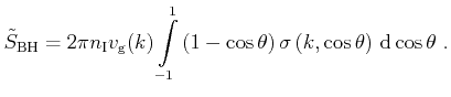
Using the potential (3.35) in Fermi's golden rule and
integrating over the final states the equivalent total scattering rate
is found to be [Kosina97]
 |
(3.51) |
Figure 3.5 shows the low field electron mobility versus the doping
concentration in Si. The Monte Carlo result is achieved by using a
modified Brooks-Herring scattering model, which includes a two-ion potential
and dispersive screening. The result shows fairly good agreement with
experimental data [Masetti83]. Further improvements can be achieved by
taking the second Born correction and plasmon scattering into
account [Kosina98].
Impact ionization is modeled using a modified threshold expression [Cartier93]
 |
(3.52) |
where
 is the impact ionization scattering rate,
 and
and
 are threshold energies, and
  and
and  are prefactors which determine the softness of the
threshold. The value of the offset energy
are prefactors which determine the softness of the
threshold. The value of the offset energy
 is chosen to render
the scattering function continuous.
is chosen to render
the scattering function continuous.
The parameters are tuned to reproduce measured electron
velocity field characteristics [Canali75] and impact ionization
coefficients [Slotboom87][Overstraeten70]
[Maes90] for relaxed Si:
 ,
,
 ,
,
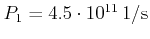 ,
,
 , and
, and
 . For strained Si the threshold values are adjusted in accordance
with the bandgap change. After an impact ionization scattering event is
evaluated the overall final energy
. For strained Si the threshold values are adjusted in accordance
with the bandgap change. After an impact ionization scattering event is
evaluated the overall final energy
 is randomly
distributed between the hole and the primary and secondary electrons.
is randomly
distributed between the hole and the primary and secondary electrons.
Fig 3.6 depicts the impact ionization coefficient of
electrons in Si as a function of the inverse electric field. The simulation
result agrees very well with various measured values from literature.
Figure 3.6:
Impact ionization coefficient
versus the inverse electric field. Monte Carlo result (VMC) is
compared to measurements [Overstraeten70] [Slotboom87][Maes90].
|
|
Next: 4. Monte Carlo Technique
Up: Dissertation Gerhard Karlowatz
Previous: 2. Strained Band Structure
G. Karlowatz: Advanced Monte Carlo Simulation
for Semiconductor Devices
![\includegraphics[width=3.6in]{xmgrace-files/MobTemp2.eps}](img353.png)
![\includegraphics[width=3.6in]{figures/fieldcmp.eps}](img366.png)
![\includegraphics[width=3.74in]{ECSfigures/highVelocityComp2.eps}](img367.png)
![\includegraphics[width=3.7in]{ECSfigures/highEnergyComp2.eps}](img368.png)
![\includegraphics[width=0.62\linewidth, clip]{figures/DopingMobSi.eps}](img400.png)
![\includegraphics[width=3.7in]{figures/IICoeff.eps}](img422.png)