During the development of numerical codes it is very important to find simple test cases for which the analytical solution is known and which can be used to debug and test the simulator.
In the bulk case we assume a constant field ![]() and constant doping.
If all quantities are space independent we
get the following system of equations:
and constant doping.
If all quantities are space independent we
get the following system of equations:
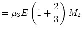
| (2.68) | ||
 |
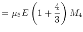
(2.69) | |
 |
(2.70) | |
|
and
| ||
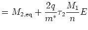 |
(2.71) | |
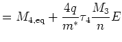 |
(2.72) | |
![]()
![]()
![]()
![]() Previous: 2.3.3 Analytical Mobility and
Up: 2.3 Closure Relations for
Next: 2.3.5 Hierarchy of Equations
Previous: 2.3.3 Analytical Mobility and
Up: 2.3 Closure Relations for
Next: 2.3.5 Hierarchy of Equations