2.3.3 Analytical Mobility and Relaxation Times

Our first implementation used a mobility model which was originally introduced by Hänsch. The higher order parameters used were found by fitting data from Monte Carlo simulations. It is a specialization of a more general model which has been implemented in MINIMOS-NT.

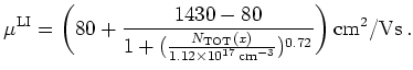
Define (lattice scattering, lattice impurity scattering):

$$\mu^{\mathrm{L}} = 1430 \mathrm{cm^2/Vs}$$ (2.58)

$$\mu^{\mathrm{LI}} = \bigg (80 + \frac{1430 - 80} {1 + (\frac{N_{\... ....12\times 10^{17} \mathrm{cm^{-3}}})^{0.72}} \bigg) \mathrm{cm^2/Vs} .$$ (2.59)

Here $N_{\mathrm{TOT}}$ is the net doping, i.e.,

$$N_{\mathrm{TOT}}(x) = \vert N_{\mathrm{D}}(x) - N_{\mathrm{A}}(x)\vert .$$ (2.60)

Then using the form

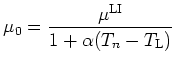$$\mu_0 = \frac{\mu^{\mathrm{LI}}}{1 + \alpha(T_n - T_{\mathrm{L}})}$$ (2.61)

where

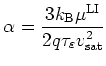$$\alpha = \frac{3 k_{\mathrm{B}}\mu^{\mathrm{LI}}}{2 q \tau_{\varepsilon} v_{\mathrm{sat}}^2}$$ (2.62)

with the saturation velocity in silicon

$$v_{\mathrm{sat}} = 10^7 \mathrm{cm/s}$$ (2.63)

we get

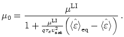$$\mu_0 = \frac {\mu^{\mathrm{LI}}} { 1 + \frac{\mu^{\mathrm{LI}}}{... ...lon \rangle }}_{\mathrm{eq}} - \hat{\langle \varepsilon \rangle } \Bigr) } .$$ (2.64)

For the higher mobilities we use

$$\mu_i = \gamma_i \mu_0$$ (2.65)

with

$$\gamma_2 \le 0.8 \quad \gamma_4 \le 0.7 .$$ (2.66)

For the relaxation times we use

$$\tau_2 = 0.33 \mathrm{ps} \quad \tau_4 = 0.2 \mathrm{ps} .$$ (2.67)

This analytical model gives good results on some practical examples. In the production version of MINIMOS-NT we take a different approach. We use tables for the mobilities and relaxation times. These tables are extracted from Monte Carlo data in such a way that the six moments model gives identical results for the bulk case. See Section 2.3.4 for details.