Disseration: Efficient Flux Calculations for Topography Simulation — Ray-Surface Intersection Tests for Particle Transport

5 Ray-Surface Intersection Tests for Particle Transport

The particle transport calculation in either bottom-up or top-down schemes relies on a large number of ray-surface intersection tests (cf. Section 2.2). The result of an intersection test is the distance from the origin of the ray to the closest intersection with the surface in the direction of the ray. Figure 5.1 illustrates two choices for the representation of a surface: An implicit representation (e.g., a signed-distance field) and an explicit representation (triangle mesh) of a sphere.

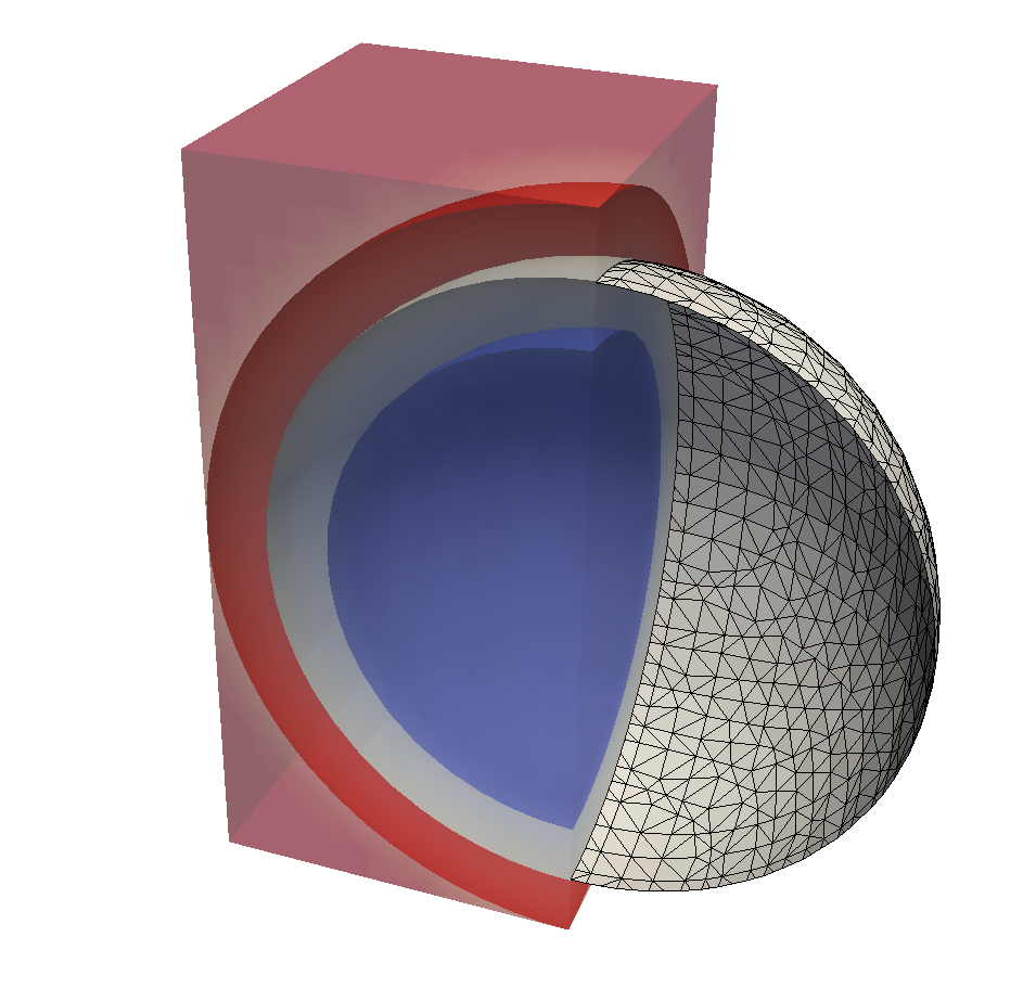
Figure 5.1: Illustration of two surface representations of a sphere: Left: Implicit representation using a signed-distance field. The blue and red surfaces are the isosurfaces delimiting the narrow-band of 3 grid cells around the interface to the inside (blue) and outside (red). The gray surface is the zero-level-set. Right: Triangle mesh extracted from the zero-level-set.

If an explicit representation of the surface is used, the intersection test identifies the closest intersection point and the corresponding primitive, e.g., a specific triangle out of a triangle mesh. A straightforward implementation is to test each primitive of a mesh for an intersection with the ray and store the resulting distance to the intersection point. Finally, the closest intersection point and the corresponding primitive is reported. The primitives need not necessarily form a closed polygonal surface, e.g., in [10] tangential disks are used and in [13] spheres are used to represent the surface.

For an implicit representation, e.g., a signed-distance field, the intersection point is a coordinate (on the isosurface) between the vertices of the grid holding the signed-distance field. A straightforward implementation is to advance a test point in steps along the ray direction. The step length is thereby equal to the absolute value of the signed-distance field at the location of the test points. The signed-distance value is then re-evaluated at the new position of the test point. The procedure is repeated until the signed-distance value changes its sign or the absolute value falls below a threshold value. The last position of the test point is then reported as the intersection point. This procedure is referred to as sphere tracing [81].

In applications requiring a high throughput of ray-surface intersections, e.g., rendering or non-imaging optics, typically a spatial data structure is constructed from the surface representation to accelerate the intersection tests. The most common data structure is a bounding volume hierarchy (BVH), which reduces the number of necessary intersection tests by grouping primitives hierarchically into bounding boxes.The intersection tests are then performed with the bounding boxes. Only if a bounding box is intersected by a ray, the hierarchically lower bounding boxes (or contained primitives) are tested for intersection. Hardware-tailored ray tracing libraries (cf. Section 2.2) originally designed for computer graphics applications provide highly-optimized ray tracing kernels for common modern computing platforms. As target applications commonly include real-time rendering of dynamic geometries, the libraries also focus on optimizing the performance of the BVH construction. Most libraries solely support single-precision arithmetics; this allows to fully utilize SIMD instructions on modern CPUs and to utilize the high single-precision processing power of GPUs.

In a feature-scale process simulator, the surface is typically represented as a narrow-band level-set (cf. Section 2.1). The most widely used approach, and thus the frame of reference for the here presented evaluations, is to perform the ray casting on the implicit representation, i.e., the level-set function. An advantage is that no explicit representation of the surface has to be extracted in each time step. However, the consequential lack of a closed polygonal explicit surface representation is disadvantageous, as the surface topology in the neighborhood of a surface point is not readily accessible, which is demanded by spatially adaptive approaches for the calculation of the particle transport (cf. Section 6.1).

In the following, an in the course of this work developed approach is presented which extracts an explicit polygonal mesh in each time step of a feature-scale simulation [2]. This mesh is then used for the ray casting during the particle transport. The underlying motivation is to utilize the higher throughput of ray-surface intersections during the particle transport; however, the overhead introduced by mesh extraction from an implicit surface representation must be considered. The ray casting is performed using single-precision arithmetic.

First, the accuracy of ray casting using single- and double-precision floating point representations is compared using a generic test scenario. Then, the performance difference for single-precision ray casting is compared using two highly optimized open-source libraries for ray casting on implicit and explicit surfaces. Finally, the newly developed approach is presented in more detail and an evaluation of the performance is presented for a simple deposition test case.

5.1 Single-Precision Ray Casting

The sufficiency of single-precision arithmetics depends on the numerical method and the further use of the result. The methods to calculate the particle transport (cf. Section 2.2) use ray casting to detect ray-surface intersections along a certain direction. The resulting information is binary and therefore the influence of the arithmetic precision of the ray casting is isolated.

To evaluate the applicability of single-precision ray casting for the ray-surface intersections during the particle transport, the angular resolutions which are achieved for single- and double-precision ray casting are compared. A spherical mesh (double-precision vertex coordinates), generated by subdividing an icosahedron 6 times (cf. Section 4.1, i.e., about $4\cdot 10^4$ vertices), serves as a reference mesh. The radius of the reference mesh is scaled from $r=10^{-16}$ to $r=10^{18}$ and rays are traced from the origin towards each vertex of the mesh. Figure 5.2 conceptually illustrates the spherical reference mesh at different scales and the corresponding rays towards the vertices of the mesh. The distance between the intersection point (found by ray casting) and the vertex coordinate on the reference mesh is computed for all vertices. The ratio of this distance and the radius $r$ provides information about the maximum angular resolution of the intersection test.

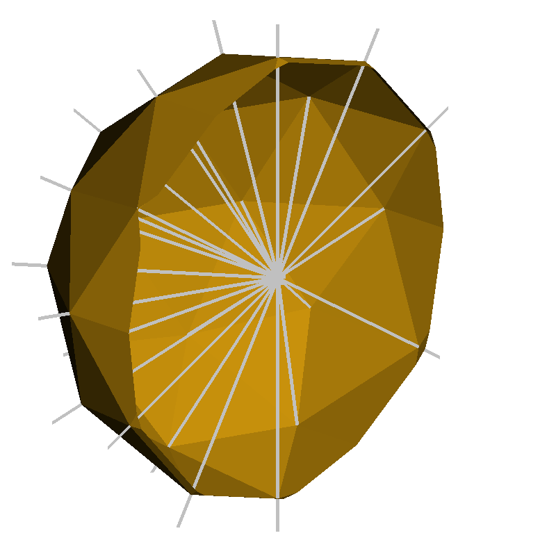
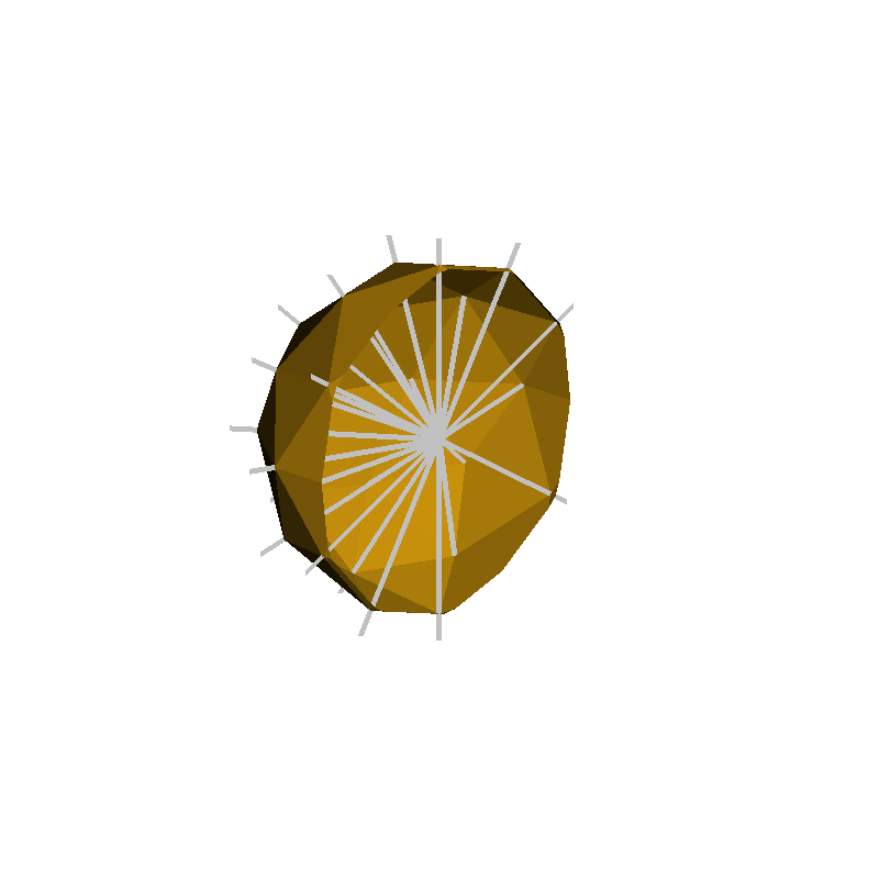
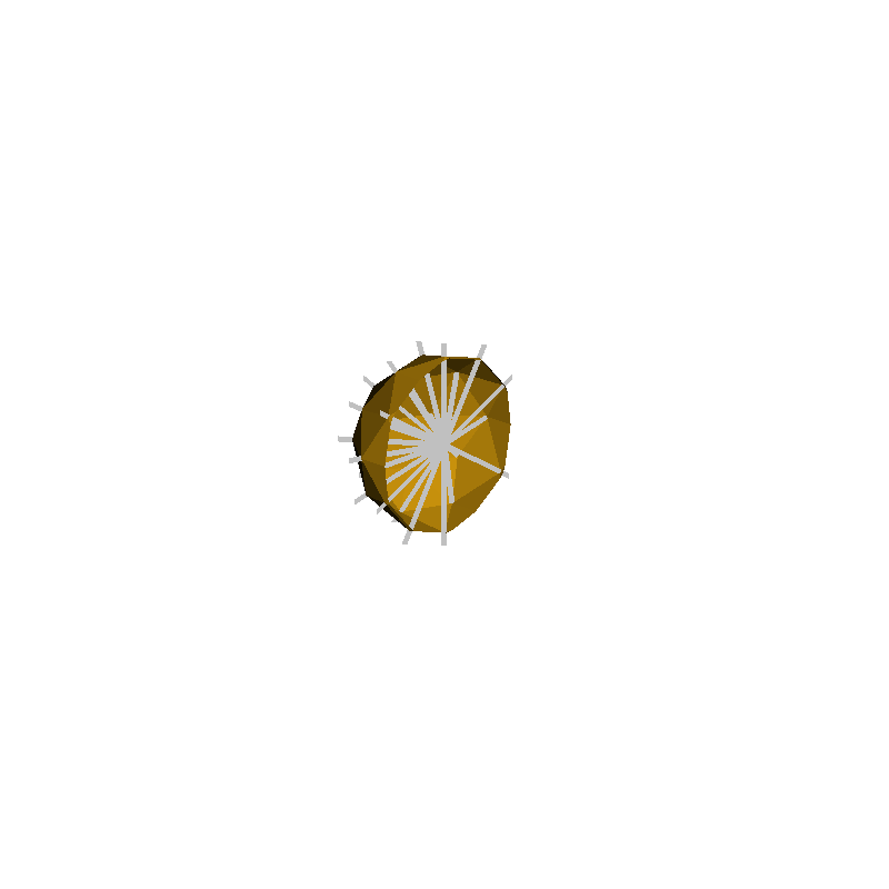
Figure 5.2: Conceptual visualization of the geometric configuration of the ray casting precision evaluation: The cross section of the spherical mesh is shown (for different scales) together with the rays which start at the origin and point into the directions of each vertex of the spherical mesh. The distance between the intersection position of each ray with the mesh (found by ray casting) and the corresponding vertex coordinate are calculated for single- and double-precision ray casting.

The NanoRT library [92] is used for single- and double-precision ray casting; the Embree library [89] is additionally used for single-precision. In Figure 5.3, the results for the maximum distance $d_{max}$ and the distance normalized to the radius $d_{norm}=d_{max}/r$ are plotted over the radius $r$ of the reference sphere. The normalized distance is constant for single- and double-precision, respectively; the constant values are $\approx 10^{-7}$ and $\approx 5\cdot 10^{-16}$ falling in the range of significant digits for single- and double-precision, respectively. For $r < 10^{-12}$ and $r > 10^{13}$ no intersection is found for single-precision ray casting using NanoRT; the same holds for Embree where the lower limit is $r < 10^{-7}$ . The angular resolution of subdivided icosahedrons (cf. Section 4.1) are indicated with dotted lines.

Figure 5.3: Evaluation of the angular resolution using single-precision (green, red) and double-precision (blue) ray casting. The maximum distance $d_{max}$ between the intersection point (found by ray casting) and the reference point is shown as solid line and the scale on the left. The normalized distance $d_{norm} = d_{max}/r$ is shown as dashed line and the scale on the right. Two lines are shown for each result which correspond to two different ways of calculating the intersection point with the mesh: (a) using a scaling of the direction of the ray with the distance of the intersection (solid for $d_{max}$ , dashed for $d_{norm}$ ) or (b) using the coordinates of the intersected primitive combined with the local intersection coordinates (dotted). Additionally, the angular resolutions of a subdivided icosahedron are shown as horizontal dotted lines for up to $n=12$ subdivisions.

$ d_{max} $ — Figure 5.3: Evaluation of the angular resolution using single-precision (green, red) and double-precision (blue) ray casting. The maximum distance $d_{max}$ between the intersection point (found by ray casting) and the reference point is shown as solid line and the scale on the left. The normalized distance $d_{norm} = d_{max}/r$ is shown as dashed line and the scale on the right. Two lines are shown for each result which correspond to two different ways of calculating the intersection point with the mesh: (a) using a scaling of the direction of the ray with the distance of the intersection (solid for $d_{max}$ , dashed for $d_{norm}$ ) or (b) using the coordinates of the intersected primitive combined with the local intersection coordinates (dotted). Additionally, the angular resolutions of a subdivided icosahedron are shown as horizontal dotted lines for up to $n=12$ subdivisions.

The results reveals that the achieved angular resolution is more than two decades smaller than the angular resolution of a 12 times subdivided icosahedron for both, single-precision and double-precision ray casting.

In conclusion, the arithmetic precision achieved with single-precision ray casting is sufficient to calculate the ray-surface intersection tests in practical three-dimensional feature-scale process simulations: For bottom-up flux calculation schemes, the angular resolution is sufficient even for the highest practical spatial sampling resolutions; the same holds for top-down flux calculation schemes. For instance, considering a cylindrical hole of aspect ratio $1000$ , i.e., depth $1000$ and diameter $1$ : Taking the area of the opening aperture $A_o = 0.5^2\pi$ and approximating a ray direction starting from the bottom of the structure with coverage $A_{ray} = (1000\cdot 10^{-7}/2)^2\pi$ on $A_o$ , the aperture can be sampled with $A_o/A_{ray} = 10^7$ ray directions. The bottom of the hole can consequently be sampled with $10^7$ rays starting at a single position on the source plane.

5.2 Ray Casting Performance for Non-Imaging Applications

In rendering applications, the ray tracing performance is commonly reported in achieved frames per second for a given scene and perspective. An alternative metric, and suitable for topography simulations in Process TCAD, are the traced rays per second, usually denoted in million rays per second (Mrays/s). The actual computations assigned to the tracing of a single ray are defined by the rendering algorithm and may include followup computations, e.g., to calculate shading. The following benchmark solely aims at evaluating the performance of the raw intersection test (i.e., the calculation of the closest intersection point with a surface) for spatially incoherent rays.

The surface is a unit sphere with $r_{unit}=1$ centered at the origin for all configurations in the following. The origins of the rays are distributed on another sphere with $r_{org} = r_{unit} + d$ ; this leads to rays which start inside the surface for $d<0$ and rays which start outside the surface for $d>0$ . At each origin, rays are traced towards the centroids of the triangles of a subdivided icosahedron (cf. Section 4.1). Figure 5.4 illustrates this benchmark scheme conceptually for two-dimensions.

Figure 5.4: Conceptual two-dimensional illustration of the benchmark scheme: The red circle represents the unit sphere and the blue dotted circles represent the spheres on which the ray origins are distributed. The black arrows indicate the scheme for the ray directions which are defined using a subdivided icosahedron. The left and right side illustrate the configurations $r_{org} < r_{unit}$ and $r_{org} > r_{unit}$ , respectively.

$ r_{org} < r_{unit} $ — Figure 5.4: Conceptual two-dimensional illustration of the benchmark scheme: The red circle represents the unit sphere and the blue dotted circles represent the spheres on which the ray origins are distributed. The black arrows indicate the scheme for the ray directions which are defined using a subdivided icosahedron. The left and right side illustrate the configurations $r_{org} < r_{unit}$ and $r_{org} > r_{unit}$ , respectively.

The performance of two open-source libraries from the field of computer graphics is compared: OpenVDB [95] is used for implicit, and Embree [89] for explicit surfaces. The rays are traced against a narrow-band level-set representation of a sphere with radius $r_{mesh}=1$ using OpenVDB’s LevelSetRayTracer and against a triangulated mesh (extracted from the level-set) using Embree. The implicit mesh is represented with OpenVDB’s default tree configuration Tree4 and a narrow-band half-width of 3 level-set grid spacings $d_{vox}$ . The for loop which iterates over the ray origins is OpenMP-parallelized. All performance measurements were performed on WS1. The benchmarks were performed using Embree 2.12, OpenVDB 4.0, and compiled using gcc 6.1.1. Table 5.1 summarizes the parameter range of the performance analysis.

$ n_{trace} $ — Table 5.1: Parameter variations used in the performance comparison (K = thousand, M = million). An active voxel is a level-set grid cell in the narrow-band level-set around the surface.

Fig 5.5 compares implicit and explicit ray casting performance for different ray origins $r_{org}$ and different surface resolutions. The limits of the achieved performance with 8 threads for Embree are about 100 Mrays/s ( $r_{org}=1.5$ , 15K triangles, Figure 5.5c) and about 10 Mrays/s ( $r_{org}=0.85$ , 6.0M triangles, Figure 5.5b). For the implicit ray casting using OpenVDB, the limits are about 13 Mrays/s ( $r_{org}=1.5$ , 0.4M triangles, Figure 5.5c) and 2 Mrays/s ( $r_{org}=0.85$ , 6.0M triangles, Figure 5.5b).

The resulting performance gain is between 3 and 6 for all possible combinations of the parameters in Table 5.1, excluding low spatial resolutions (i.e., less than 0.4 million triangles). The performance gain is higher for the multi-threaded runs, the main reason being the higher speedup for Embree in the hyper-threading regime (cf. Figure 5.6). For low spatial resolutions (less than 0.4 million triangles) the performance ratio is increasing. For high spatial resolutions (i.e, more than 1 million triangles) the multi-threaded performance ratio is $\approx 3.5$ for $r_{org}<1$ and $\approx 4.5$ for $r_{org}>1$ , i.e., Embree profits more than OpenVDB if a large portions of the rays do not intersect the geometry at all.

$ r_{org}<1 $ — (a) 1 thread, $r_{org}<1$

Fig 5.6 plots the achieved speedup for the parallelized for loop (which iterates over the ray origins) for explicit and implicit ray casting. Both parallelizations show nearly an ideal speedup for 2 threads. The speedup spreads for 4 threads with a minimum speedup of 2.7 (Embree) and 2.0 (OpenVDB). The speedup for 8 threads is up to 6 for Embree and up to 5 for OpenVDB. The parameter combinations which show nearly no speedup between 2 to 4 threads (cf. Figure 5.6b) were identified to have a low hit ratio ( $\text {number of hits}/\text {number of traced rays } < 0.13$ ) and a large voxel size ( $d_{vox} >= 0.01$ ). For 5 and more threads (entering the hyper-threading regime) this influence is compensated leading to an overall speedup between 3 and 4 for 6 threads.

5.3 Temporary Explicit Meshes for
Flux Calculation

Based on the results from the previous sections a scheme is introduced which aims to accelerate the particle transport calculation of a level-set-based process simulation. It bases on the extraction of a temporary explicit surface mesh (from the level-set) in each time step of the simulation. Figure 5.7a and 5.7b illustrates the sequence of computational tasks in a time step of a level-set-based process simulation.

The scheme introduces new computational tasks for each time step, namely

• the extraction of the explicit surface mesh from the level-set,
• the generation of an acceleration structure (for efficient intersection tests) from the extracted mesh, and
• the interpolation of the surface rates from the explicit mesh to the positions of the level-set grid (computationally negligible).

Using the libraries benchmarked in Section 5.2 the overhead introduced by the approach is estimated. Figure 5.7c plots the runtime on WS1 (8 threads) for the generation of the temporary explicit mesh and the construction of the acceleration structure, when using OpenVDB to represent the level-set and to extract the mesh, and the acceleration structure of Embree. Different resolutions of the unit sphere (analog to the benchmarks above) are tested; the maximum runtime is identified with a total of less than 1.4 seconds for a mesh with about 6 million triangles. The overhead per million triangles is about 0.2 seconds for meshes with more than 0.4 million triangles.

Performance Evaluation

The simulation platform described in Section 3 is used to implement a simple deposition test case: A cube with edge length $1.5$ is centrally placed in a $2 \times 2$ domain with periodic boundary conditions. The direct flux $F$ from an ideal-diffuse source is calculated and a simple linear deposition $V_n = F$ is used as surface velocity model. The direct flux is calculated using a bottom-up scheme with a 4 times subdivided icosahedron (cf. Section 4.1) to sample the spherical directions. The lateral level-set resolution is set to $128 \times 128$ and the resulting explicit surface meshes for the initial and final geometry count about $150$ K and $250$ K triangles, respectively. Figure 5.8 illustrates the initial, intermediate, and final geometry of the deposition simulation.

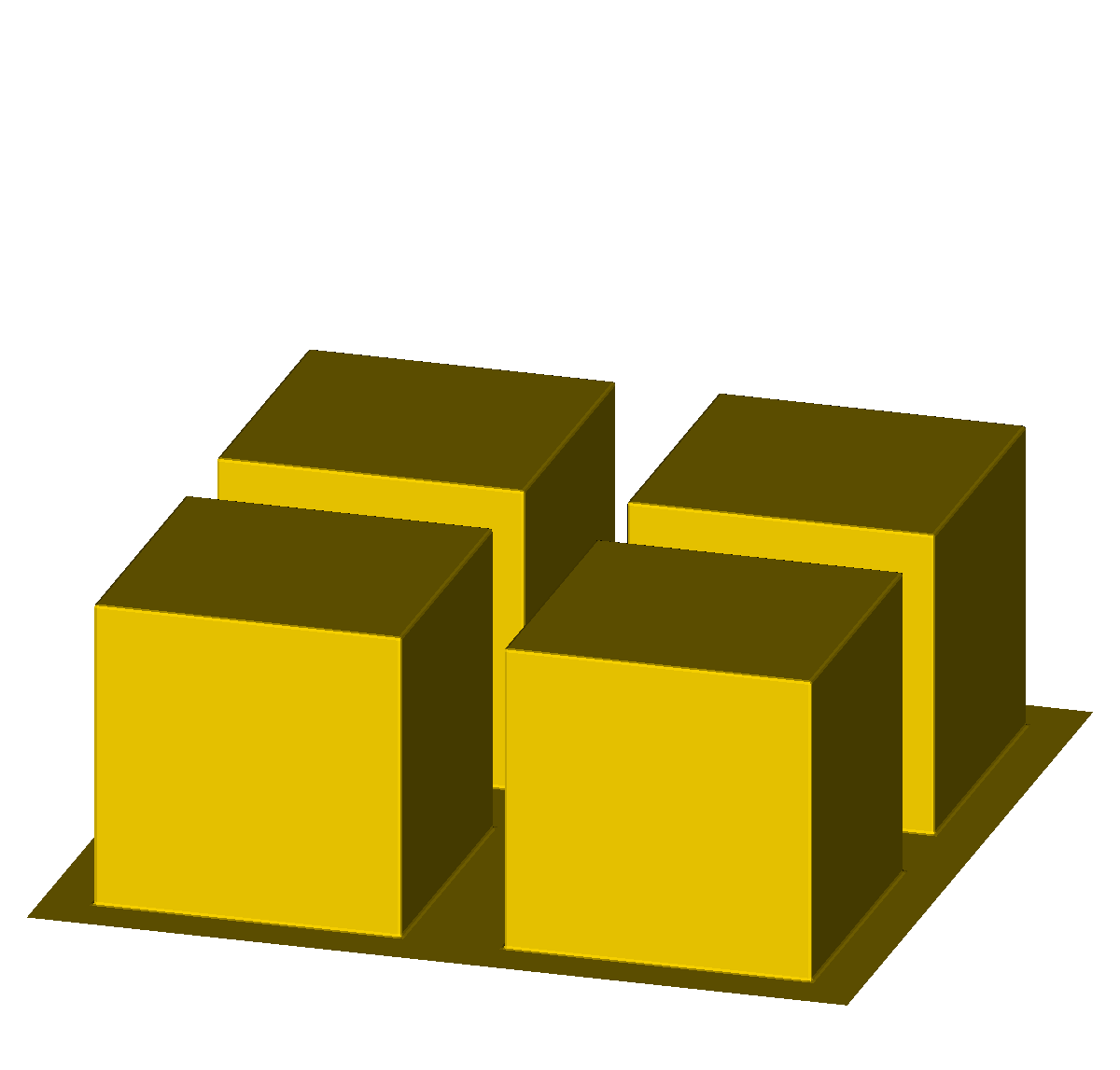
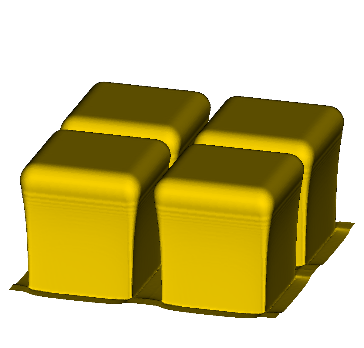
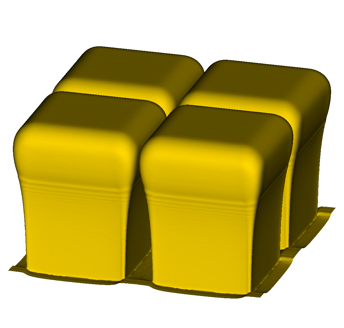
Figure 5.9 shows the runtime of the main computational tasks throughout the simulation. The runtime for the calculation of the surface rates (i.e., the direct flux calculation in this case) is dominating for both simulations. Nevertheless, the speedup is about 7 to 9 when using explicit ray tracing. The speedup is in accordance with the estimates of the generic benchmark in Section 5.2. However, differently to the benchmark above, the ray origins are located near the surface, i.e., they start inside the narrow-band of the level-set. Considering the geometry visualized in Figure 5.8c, it is apparent that most rays start in the narrow-band and intersect the narrow-band. This configuration is not considered in the benchmark above, where all ray origins are located at some distance to the narrow-band.

5.4 Summary

Single-precision ray tracing is attested sufficient accuracy, for top-down and bottom-up approaches for the particle transport in practical simulation scenarios.

The ray casting performance when using OpenVDB for implicit surfaces and Embree for explicit surface representations is studied using a generic test for non-imaging application. The performance gain is at minimum a factor of 3 for a wide range of scenarios.

An approach to perform the ray-surface intersections not on the level-set-based implicit representation of the surface but on a temporary explicit mesh was presented and compared. The performance gain in a deposition test case using a bottom-up approach to calculate the direct flux is a factor between 7 and 9 using the benchmarked libraries.