Next: B. Layout Data Formats
Up: A. Basis of the
Previous: A.1 The GAUSSIAN Normal
Subsections
Let
 be a set of
  independent random variates and
  have an arbitrary probability distribution
 with
mean
with
mean  and a finite variance
 .
.
Two variates A and B are statistically independent if the conditional
probability
 (probability of an event A
assuming that B has occurred) of A given B satisfies
(probability of an event A
assuming that B has occurred) of A given B satisfies
 |
(A.15) |
in which case the probability of A and B is just
 |
(A.16) |
Similarly, n events
 are independent if
 |
(A.17) |
Then the normal form variate
 |
(A.18) |
has a limiting cumulative distribution function which approaches a normal
distribution.
Under additional conditions on the distribution of the variates, the
probability density itself is also normal with mean  and variance
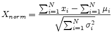
 . If conversion to normal form is not performed, then the
variate
. If conversion to normal form is not performed, then the
variate
 |
(A.19) |
is normally distributed with
 and
and
 .
.
Consider the inverse FOURIER transform of  .
.
Now write
 |
(A.21) |
 |
(A.22) |
so we have
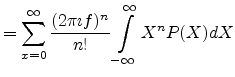
Now expand
 |
(A.24) |
so
since
 |
(A.26) |
 |
(A.27) |
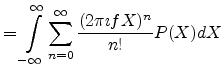
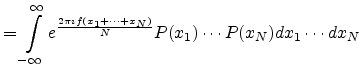
Taking the FOURIER transform
![$\displaystyle P_X \equiv \int_{-\infty}^{\infty} e^{-2 \pi \imath f x} {\cal F}^{-1}\left[P_X(f)\right] df$](img403.png) |
|
 |
(A.28) |
This is of the form
 |
(A.29) |
where
 and
and
 . This integral yields
 |
(A.30) |
Therefore
But
 and
, so
and
, so
 |
(A.32) |
The ``fuzzy'' central limit theorem says that data which are influenced by
many small and unrelated random effects are approximately normally distributed.
Next: B. Layout Data Formats
Up: A. Basis of the
Previous: A.1 The GAUSSIAN Normal
R. Minixhofer: Integrating Technology Simulation
into the Semiconductor Manufacturing Environment
 \equiv \int_{-\infty}^{\infty} e^{2 \pi \imath f X} P(X) dX$](img382.png)
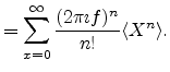
 = \sum_{x=0}^\infty \frac{(2 \pi \imath f)^2}{n!} \langle X^n \rangle$](img388.png)
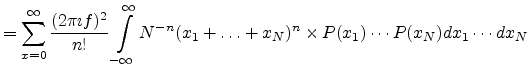
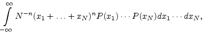
![$\displaystyle = \int_{-\infty}^{\infty} \sum_{n=0}^{\infty}\left[\frac{2 \pi \i...
...+ \ldots + x_N)}{N}\right]^n \frac{1}{n!} P(x_1) \cdots P(x_N) dx_1 \cdots dx_N$](img390.png)
![$\displaystyle = \left[\int_{-\infty}^{\infty} e^{\frac{2 \pi \imath f x_1}{N}} ...
...eft[\int_{-\infty}^{\infty} e^{\frac{2 \pi \imath f x_N}{N}} P(x_N) dx_N\right]$](img392.png)
![$\displaystyle = \left[\int_{-\infty}^{\infty} e^{\frac{2 \pi \imath f x}{N}} P(x) dx\right]^N$](img393.png)
![$\displaystyle = \left\{ \int_{-\infty}^{\infty}\left[1+\left(\frac{2 \pi \imath...
...\left(\frac{2 \pi \imath f}{N}\right)^2 x^2 + \ldots \right] P(x) dx \right\}^N$](img394.png)
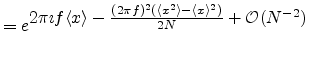
![$\displaystyle = \left[1+\frac{2 \pi \imath f}{N} \langle x \rangle - \frac{(2 \pi f)^2}{2 N^2} \langle x^2 \rangle + {\cal O}(N^{-3})\right]^N$](img395.png)
![$\displaystyle = e^{\textstyle N \ln{\left[1+\frac{2 \pi \imath f}{N} \langle x ...
...le - \frac{(2 \pi f)^2}{2 N^2} \langle x^2 \rangle + {\cal O}(N^{-3})\right]}}.$](img396.png)
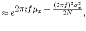
 \approx e^{\textstyle N \left[\frac{2 ...
...}{2}\frac{(2 \pi \imath f)^2}{N^2} \langle x \rangle^2+{\cal O}(N^{-3})\right]}$](img398.png)
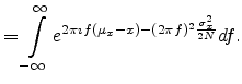
![$\displaystyle P_X = \sqrt{\frac{\pi}{\frac{(2 \pi \sigma_x)^2}{2N}}} e^{\textstyle \frac{-[2 \pi (\mu_x - x)]^2}{4 \frac{(2 \pi \sigma_x)^2}{2N}}}$](img409.png)