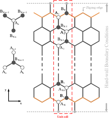
Figure 4.1: The structure of a GNR with zigzag edges along the x direction.
Each unit cell consists of N atomes at the sublattice A or B. A hard wall
boundary condition is imposed on the both edges.
The structure of graphene consists of two types of sublattices A and B, see Fig. 4.1.
We start with the Hamiltonian (Eq. 3.6) and wave functions (Eq. 3.18 and Eq. 3.19) of graphene and derive the analytical expressions for ZGNRs.
To obtain ϕp in wave functions |ψA| and |ψB|, one can substitute the ansatz for the wave functions into the Schr¨odinger equation. An A-type carbon atom at some atomic site n has one B-type atom at some atomic site N - n and two B-type neighbors at N - n + 1, see Fig. 4.1:
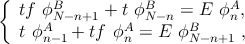 | (4.1) |
replacing the index n with n + 1 in the second relation of Eq. 4.1, one obtains:
 | (4.2) |
Substituting this relation in Eq. 4.1 one can rewrite Eq. 4.1 as:
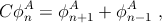 | (4.3) |
with:
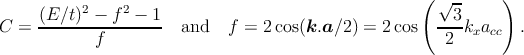 | (4.4) |
Due to symmetry, a similar relation holds for the B-type carbon atoms:
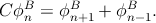 | (4.5) |
Considering the boundary condition ϕ0A = ϕ 0B = 0, the solution to the recursive formula is given by (see Appendix B.2):
 | (4.6) |
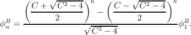
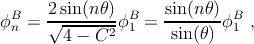
Depending on the values of C, Eq. 4.4 can have three different solutions. For |C| > 2, ϕnB has a hyperbolic solution where the wave function is localized at the edges of the ribbon:
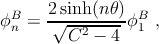 | (4.7) |
where θ is given by:
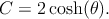 | (4.8) |
For C = ±2, the amplitude of the wave function increases linearly with n. This
critical case appears at the transition point from localized states to delocalized
states. For |C| < 2 ,  is a pure imaginary number. The solution ϕnB is,
therefore, given by:
is a pure imaginary number. The solution ϕnB is,
therefore, given by:
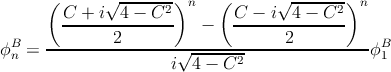 | (4.9) |
 | (4.10) |
where θ is the wavenumber and is given by
 | (4.11) |
Under this condition the wave function has an oscillatory behavior and is not localized.
The prefactors CA and CB in Eq. 3.18 are found to be CA = ±CB, see Appendix B.1. To simplify the equations we assume ϕ1A∕B = sin(θ).
Therefore, the wave functions become
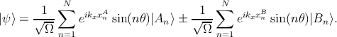 | (4.12) |
To obtain the normalization factor Ω, one has to impose the following condition [168] in the Eq. 3.19:
 | (4.13) |
By substuting Eq. 4.12 in Eq. 4.13 one obtains
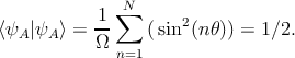 | (4.14) |
It is straightforward to obtain ΩA∕B = Ω as
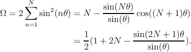 | (4.15) |
In principle θ can not be derived analytically for ZGNRs. However, two approximations for θ are discussed in Sec. 4.2. Using the analytical approximated θ calculated in Eq. 4.28, Eq. 4.15 can be simplified as
 | (4.16) |
In order to obtain the respective energy spectrum, Eq. 4.4 can be written as
![E = ±t [Cf + f2 + 1]1∕2.](diss122x.png) | (4.17) |
By substituting Eq. 4.4 and Eq. 4.11 in Eq. 4.17, the energy dispersion relation takes the form
![[ ( √ -- ) ( √-- ) ]1∕2
E = ±t 1 + 4 cos2 --3k a + 4cos -3-k a cos(θ) .
2 x cc 2 x cc](diss123x.png) | (4.18) |