3.5.6.1 Particle Flux Equation

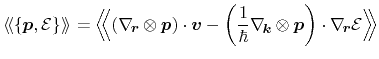
In the following, the derivation of the particle flux equation is performed analogously to Stratton's approach. The starting point is again the Boltzmann transport equation with a general weight $\ensuremath{\ensuremath{\mathitbf{X}}}$ in the form of equation (3.30). Inserting $\ensuremath{X} = \ensuremath{\ensuremath{\mathitbf{p}}}$ as $\ensuremath{X}$ yields

$$\underbrace{\vphantom{\frac{1}{\hbar}}\ensuremath{\ensuremath{\en... ...le \! \rangle}}{\ensuremath{{\tau_\ensuremath{\ensuremath{\mathitbf{j}}}}}} \,.$$ (3.80)

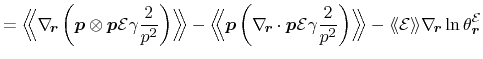
Application of the trace approximation of tensor valued expressions (3.39) as well as a product ansatz for the energy as presented in equation (3.40) on term (i) results in

$$\ensuremath{\ensuremath{\ensuremath{\mathitbf{\nabla_{\!r}}}}}\en... ... \! \langle \ensuremath{\mathcal{E}}\ensuremath{\gamma} \rangle \! \rangle} \,.$$ (3.81)

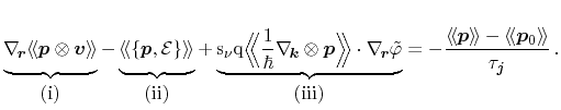
The Poisson bracket within the average in (ii) has to be expanded using (A.6). Furthermore, the inverse product rule (B.3) is used to transform the $\ensuremath{\ensuremath{\ensuremath{\mathitbf{\nabla_{\!r}}}}\ensuremath{\otimes}}\ensuremath{\ensuremath{\mathitbf{p}}}$ - term in the first term. The product ansatz for the energy as well as the trace approximation result in

$$\ensuremath{\langle \! \langle \ensuremath{\{\ensuremath{\ensurem... ...hitbf{\nabla_{\!r}}}}}\ensuremath{\mathcal{E}} \Bigr\rangle \! \! \Bigr\rangle}$$ (3.82)

$$= \ensuremath{\langle \! \langle \ensuremath{\ensuremath{\ensurem... ...uremath{\theta_\ensuremath{\ensuremath{\mathitbf{r}}}^\ensuremath{\mathcal{E}}}$$

$$= \ensuremath{\Bigl\langle \! \! \Bigl\langle \ensuremath{\ensure... ...uremath{\theta_\ensuremath{\ensuremath{\mathitbf{r}}}^\ensuremath{\mathcal{E}}}$$

$$= - \ensuremath{\langle \! \langle \ensuremath{\mathcal{E}} \rang... ...ath{\theta_\ensuremath{\ensuremath{\mathitbf{r}}}^\ensuremath{\mathcal{E}}} \,.$$

The third term (iii) can be handled in a straight-forward manner. Assembly of all three terms leads to

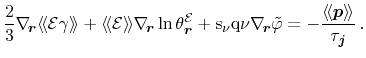
$$\frac{2}{3} \ensuremath{\ensuremath{\ensuremath{\mathitbf{\nabla_... ...le \! \rangle}}{\ensuremath{{\tau_\ensuremath{\ensuremath{\mathitbf{j}}}}}} \,.$$ (3.83)

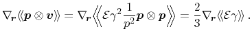
Assuming parabolic bands and a heated, displaced Maxwellian, $\ensuremath{\gamma}$ becomes unity and the average reads

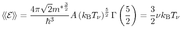
$$\ensuremath{\langle \! \langle \ensuremath{\mathcal{E}} \rangle \... ...{3}{2} \ensuremath{\nu}k_\ensuremath{\mathrm{B}}\ensuremath{T_\ensuremath{\nu}}$$ (3.84)

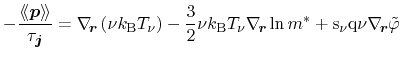
normalized with the carrier concentration (3.54). Summation over all parts as well as the mobility definition consistent with the homogeneous case

$$\ensuremath{\ensuremath{\mu}_\nu}= \frac{\mathrm{q}\ensuremath{{\tau_\ensuremath{\ensuremath{\mathitbf{j}}}}}}{m^*}$$ (3.85)

yields the final form of the particle current equation

$$- \frac{\ensuremath{\langle \! \langle \ensuremath{\ensuremath{\m... ...{\ensuremath{\ensuremath{\mathitbf{\nabla_{\!r}}}}}\ensuremath{\tilde{\varphi}}$$ (3.86)

$$\ensuremath{\ensuremath{\mathitbf{j}}_\nu}= -\frac{k_\ensuremath{... ...nsuremath{\ensuremath{\mathitbf{\nabla_{\!r}}}}}\ensuremath{\tilde{\varphi}}\,.$$ (3.87)

Rewriting the particle current equation with the electrochemical potential defined in Eqs. (3.60) and (3.62) results in

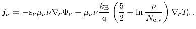
$$\ensuremath{\ensuremath{\mathitbf{j}}_\nu}= - \ensuremath{\mathrm... ...remath{\ensuremath{\mathitbf{\nabla_{\!r}}}}}\ensuremath{T_\ensuremath{\nu}}\,.$$ (3.88)

M. Wagner: Simulation of Thermoelectric Devices