Similarly as presented in Section 4.1
the matrices
![]() ,
,
![]() and
and
![]() and the right hand
side vector
and the right hand
side vector
![]() are assembled from the corresponding element matrices for
each tetrahedron Fig. <4.7>. For the first term on the right hand side
of (5.38) the rotor operator must be applied to the element edge
functions
are assembled from the corresponding element matrices for
each tetrahedron Fig. <4.7>. For the first term on the right hand side
of (5.38) the rotor operator must be applied to the element edge
functions
![]() . For the first one,
. For the first one,
![]() , it can be written
, it can be written
 |
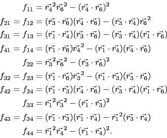
Analogously the rotor operator of all element edge functions can be expressed by
Thus the element matrix of the first term on the right hand side of (5.38) can be given by the expression
In (5.53) it is assumed that ![]() is scalar and constant at each element. A constant elemental
is scalar and constant at each element. A constant elemental
![]() is not an essential restriction, since the simulation
domain is discretized sufficiently fine, which is anyway
necessary for an accurate result. In
regions, in which it is expected that
is not an essential restriction, since the simulation
domain is discretized sufficiently fine, which is anyway
necessary for an accurate result. In
regions, in which it is expected that ![]() will seriously
change, it can be required that a finer mesh is used.
will seriously
change, it can be required that a finer mesh is used.
For the second term of (5.38) the following elemental matrix is regarded
 |
(5.54) |
 |
(5.55) |
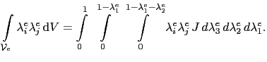
![$\displaystyle \int_{\mathcal{V}_e}\lambda^e_i\lambda^e_j \mathrm{d}V, i\in[1;4] j\in[1;4].$](img498.gif) |
 |
(5.56) |
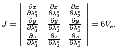
Using (4.79) the Jacobi matrix is given by the expression
Thus the integral above results in
![$\displaystyle \int_{\mathcal{V}_e}\lambda^e_i\lambda^e_j \mathrm{d}V = \left\{...
...m} & \frac{V_e}{10}, & i = j \end{array} \right. , i\in[1;4], j\in[1;4]$](img501.gif) |
(5.58) |
and ![]() can now be expressed as
can now be expressed as
 |
(5.59) |
 |
(5.60) |
 |
(5.61) |
 |
(5.62) |
 |
(5.63) |
 |
(5.64) |
| (5.65) |
with
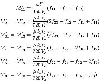
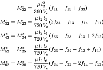
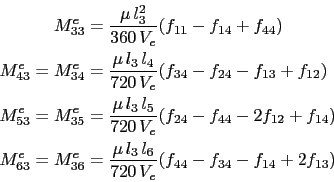
Thus the entries of the matrix ![]() are given by
are given by
The matrix with the partial derivatives
is usually called stiffness matrix and is notated with ![]() . The matrix which does
not contain any derivatives is the mass matrix
. The matrix which does
not contain any derivatives is the mass matrix ![]() . However, the designations
. However, the designations
![]() and
and ![]() come from the field of mechanics and bear on scalar fields. Analogously
in (5.67) the same notations
come from the field of mechanics and bear on scalar fields. Analogously
in (5.67) the same notations ![]() and
and ![]() are used
for the derivative and non-derivative matrix, this time for the vector field
are used
for the derivative and non-derivative matrix, this time for the vector field ![]() .
.
For element wise assembling of the matrix ![]() from (5.39),
it is also assumed that the magnetic
permeability
from (5.39),
it is also assumed that the magnetic
permeability ![]() is constant in each element. The first entry is calculated in the
following way
is constant in each element. The first entry is calculated in the
following way
The remaining entries are obtained analogously. The integral expressions in (5.68) are computed using the integral domain transformation (A.9) and (A.10) from Appendix A, where the Jacobi matrix is calculated from (4.79) and given by (5.57)
![$\displaystyle \int_{\mathcal{V}_e}\lambda^e_i \mathrm{d}V = 6V_e\int_0^1 \i...
...bda^e_i d\lambda^e_3 d\lambda^e_2 d\lambda^e_1 = \frac{V_e}{4}, i\in[1;4].$](img515.gif) |
(5.69) |
Now the entries of the element matrix ![]() can be expressed as
can be expressed as
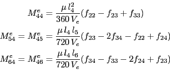
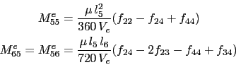
![\begin{displaymath}\begin{split}B^e_{1j} & = \frac{\mu l_1}{144 V_e}(f_{2j} - ...
... l_6}{144 V_e}(f_{4j} - f_{3j}), j\in[1;4], \end{split}\end{displaymath}](img517.gif) |
(5.70) |
where ![]() are given by (5.66).
are given by (5.66).
The matrix ![]() from (5.40) is assembled from the element
matrix
from (5.40) is assembled from the element
matrix ![]() . The entries of
the element matrix
. The entries of
the element matrix ![]() are obtained from (5.40)
are obtained from (5.40)
| (5.71) |
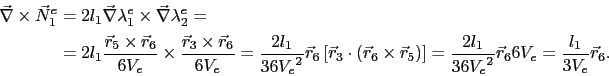
![$\displaystyle \vec{\nabla}\times\vec{N}^e_i = \frac{l_i}{3V_e} \vec{r}_{7-i}, i\in[1;6].$](img490.gif)
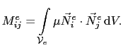
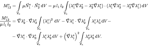
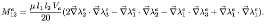
![\begin{displaymath}\begin{split}S^e_{ij} & = \int_{\mathcal{V}_e}\left(\vec{\nab...
..._{7-i}\cdot\vec{r}_{7-j}, i\in[1;6], j\in[1;6]. \end{split}\end{displaymath}](img491.gif)
![\begin{displaymath}\begin{split}B^e_{11} & = \mu\int_{\mathcal{V}_e}\vec{N}^e_1\...
...int_{\mathcal{V}_e}\lambda^e_2 \mathrm{d}V\right]. \end{split}\end{displaymath}](img514.gif)