


Next: 1.3.3 EM Lifetime Extrapolation
Up: 1.3 Empirical and Semi-Empirical
Previous: 1.3.1 Black's Equation
EM experiments normally use a given resistance increase as failure criterion.
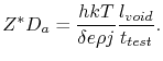
For a void spanning the entire cross sectional area of a line, the total resistance of a damascene line, as shown in Figure 1.5, is given by
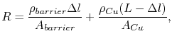 |
(1.8) |
where
 is the electrical resistivity and
 is the cross sectional area of the barrier layer,
 is the electrical resistivity and
  is the cross sectional area of the copper line,
  is the line length, and
  is the length of the void.
Thus, this equation relates resistance increase with void size.
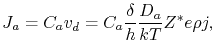
In turn, void size is connected to mass transport, which is expressed in the form [57]
is the length of the void.
Thus, this equation relates resistance increase with void size.
In turn, void size is connected to mass transport, which is expressed in the form [57]
 |
(1.9) |
where  is the atomic concentration,
 is the drift velocity,
 is the width of the interface which controls mass transport,
  is the line height,
  is the atomic diffusivity of the interface which dominates the EM transport,
  is the effective valence,
  is the elementary charge,
 is the electrical resistivity, and
 is the current density.
Figure 1.5:
Void growth in a single-damascene copper interconnect.
|
|
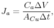
The atomic flux can also be written as [22]
 |
(1.10) |
where  is the change of the void volume in a time
  .
Combining (1.9) and (1.10) yields
.
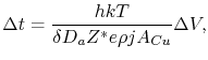
Combining (1.9) and (1.10) yields
 |
(1.11) |
so that a given test time  is related to the void volume
  ,
,
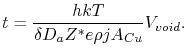 |
(1.12) |
Equation (1.12) is commonly used for estimation of the void growth time. In turn, a critical void volume is related to the line resistance according to (1.8).
Thus, the time to failure for a given resistance increase criterion can be determined.
An interesting application of such an approach was performed by Hauschildt et al. [20,22]. For a void spanning the entire line width,  , and assuming a rectangular void shape, the void volume becomes
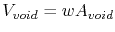 , and (1.12) yields
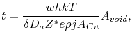 |
(1.13) |
where  is the area of the void, which can be measured using SEM pictures.
EM tests were then carried out and stopped after a given test time (called t-based by the authors) or after a certain resistance increase (R-based). In both cases, the void area mean value and standard deviation were determined. For the R-based tests the mean time to failure
is the area of the void, which can be measured using SEM pictures.
EM tests were then carried out and stopped after a given test time (called t-based by the authors) or after a certain resistance increase (R-based). In both cases, the void area mean value and standard deviation were determined. For the R-based tests the mean time to failure  can be determined which, in turn, can be used for the t-based experiments.
Finally, using the void area statistical distribution of both tests and applying (1.13) a new distribution is obtained following [20,22]
can be determined which, in turn, can be used for the t-based experiments.
Finally, using the void area statistical distribution of both tests and applying (1.13) a new distribution is obtained following [20,22]
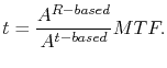 |
(1.14) |
Hence, once the statistics of the void area distribution for both test types is known, the distribution of the EM lifetimes can be estimated.
Equation (1.9) is also commonly used to extract the diffusivity from void drift experiments [57]. The drift velocity of the void boundary in Figure 1.5 is
 |
(1.15) |
which for a given test time  with a corresponding void length
  can be rearranged as
 |
(1.16) |
Since can be expressed by an Arrhenius relationship, the activation energy for diffusion can be extracted from a plot
 versus
  [38].
[38].
Next: 1.3.3 EM Lifetime Extrapolation
Up: 1.3 Empirical and Semi-Empirical
Previous: 1.3.1 Black's Equation
R. L. de Orio: Electromigration Modeling and Simulation
![\includegraphics[width=0.50\linewidth]{chapter_introduction/Figures/void_growth.eps}](img110.png)