


Next: 2.2 Diffusivity Paths
Up: 2. Physics of Electromigration
Previous: 2. Physics of Electromigration
2.1 The Electromigration Driving Force
Electromigration is the atomic migration caused by the action of microscopic forces on mobile defects. These microscopic forces arise due to the local electric field and electron transport in a conductor [58].
Typically, atomic diffusion is a random process, in the sense that there is no preference in the direction of atomic jumps [59].
However, in the process of making an atomic jump, when the atom is in the saddle point and it is out of the lattice equilibrium position, it is subject to a larger electron scattering, in such a way that the momentum transfer from the electron to the atom biases the atomic jump in the direction of the electron flow [60,61]. The force caused by this momentum transfer from the electron to the atom ion is the so-called ``wind force''.
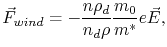
Using a semiclassical ballistic model of scattering, Huntington and Grone [1] derived for the wind force
 |
(2.1) |
where  is the density of conduction electrons,
  is the density of defects,
 is the defect resistivity,
 is the metal resistivity,
  and
and  are the free-electron mass and effective electron mass, respectively,
  is the elementary charge, and
 is the macroscopic electric field.
Upon deriving this equation, Huntington and Grone [1] assumed that the electrons are scattered by the atomic defects alone and that the defects are decoupled from the lattice.
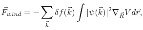
A more general expression for the wind force is given by quantum mechanics theory [62]
is the macroscopic electric field.
Upon deriving this equation, Huntington and Grone [1] assumed that the electrons are scattered by the atomic defects alone and that the defects are decoupled from the lattice.
A more general expression for the wind force is given by quantum mechanics theory [62]
 |
(2.2) |
where  is the electron-point defect interaction potential and
 is the electron scattering wave function for an electron incident upon the defect complex.
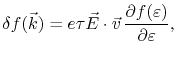
 is the perturbed electron distribution function caused by the applied field, which has the form [62]
 |
(2.3) |
where  is the transport relaxation time,
 is the velocity, and
 is the energy of an electron.
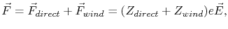
In addition to the wind force, there is a second contribution to the force acting on an atom due to the direct action of the macroscopic electric field on the migration ion, the so-called ``direct force'' [63].
Therefore, the total driving force acting on a metal ion can be written as the sum of the direct force and the wind force,
 |
(2.4) |
where  is the direct valence,
  is the wind valence.
The direct valence is the nominal valence of the metal, when screening effects are neglected. However, much controversy has appeared, when screening effects are taken into account [63]. In turn, accounts for the magnitude and direction of the momentum exchange between the conducting electrons and the metal ions.
is the wind valence.
The direct valence is the nominal valence of the metal, when screening effects are neglected. However, much controversy has appeared, when screening effects are taken into account [63]. In turn, accounts for the magnitude and direction of the momentum exchange between the conducting electrons and the metal ions.
It is convenient to write equation (2.4) as
 |
(2.5) |
where
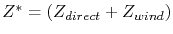 is called effective valence.
In this way, the microscopic, quantum mechanical effects of the electromigration phenomenon are comprised in the effective valence parameter, which can be theoretically calculated and experimentally measured [1,61,62,64,65,66,67]. Table 2.1 shows the effective valence values for metals commonly used in interconnect structures close to their melting temperature [67].
is called effective valence.
In this way, the microscopic, quantum mechanical effects of the electromigration phenomenon are comprised in the effective valence parameter, which can be theoretically calculated and experimentally measured [1,61,62,64,65,66,67]. Table 2.1 shows the effective valence values for metals commonly used in interconnect structures close to their melting temperature [67].
Table 2.1:
Wind and effective valence values.
| Metal |
Calculated |
Measured  |
| Al |
-3.11 |
-3.4 |
| Al(Cu) |
-5.29 |
-6.8 |
| Cu |
-3.87 |
-5.0 |
| Ag |
-3.51 |
-8.0 |
| Ta |
0.35 |
- |
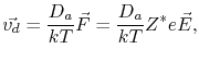
Using the Nernst-Einstein relation, the drift velocity,
 , of metal atoms and the atomic flux due to electromigration are calculated, respectively, by
 |
(2.6) |
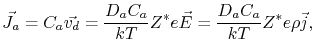
and
 |
(2.7) |
where  is the atomic diffusivity,
  is the atomic concentration,
  is Boltzmann's constant, and
  is the temperature.
The last equality in (2.7) is written in terms of the current density
is the temperature.
The last equality in (2.7) is written in terms of the current density
 , since
 .
.
From (2.6) and (2.7) one can see that the sign of the effective valence determines the direction of atomic migration. A negative value means that the atoms diffuse in a direction opposite to the external electric field, or current density, i.e. in the same direction of the electron flow.
Also, the mass flow is directly proportional to the current density and to the atomic diffusion coefficient. This means that the total material transport due to electromigration is a function of the available atomic diffusivity paths.
Next: 2.2 Diffusivity Paths
Up: 2. Physics of Electromigration
Previous: 2. Physics of Electromigration
R. L. de Orio: Electromigration Modeling and Simulation